Introduction
UNEX is a programming environment for investigation of molecular structure. I develop new and existing experimental methods and combine them in order to increase the accuracy and precision of results. At the current stage the full support of gas electron diffraction (GED [1, 2, 3]) method is provided, from the calibration of instruments and data reduction to the refinement of molecular structure. Additionally, rotational constants from microwave [4] and high-resolution molecular spectroscopy [5] can be used solely or in combination with GED data for determination of molecular geometry.
|
Cite UNEX as
Yury V. Vishnevskiy, 2023, UNEX 1.7, https://unex.vishnevskiy.group [latest access date] |
|
UNEX is not related to any version of KCED or other programs. This is an independent research project. Nevertheless, many implemented in UNEX methods and algorithms are based on investigations of other authors, see respective references for details. |
|
The aim of this manual is not to teach how to investigate molecules but only to describe UNEX functionality. Please remember that incorrect settings and inappropriate usage of different methods can lead to incorrect results! |
|
If you are reading an offline version of this manual, it may well be already outdated. Check the online version, when in doubt! |
General ideas
-
Exploration of experimental possibilities for investigation of molecular structure.
-
Development of the gas electron diffraction (GED) method and its automation.
-
Development of spectroscopic methods for molecular structure investigation.
-
Providing the ability to carry out very accurate studies due to extended facilities and flexibility of the program interface.
-
Elaboration of joint methods for molecular structure investigations.
Capabilities
-
Investigation of molecular structure by means of GED method.
-
Refinement of geometrical parameters from rotational constants.
-
Combined refinements on the basis of GED data and rotational constants.
-
Flexible restraints and rigid constraints may be applied to model parameters.
-
Semi-rigid and one-dimensional dynamic models in GED.
-
Numerical and analytical parametric forms of potential functions.
-
Support for relaxation of geometrical parameters, amplitudes and corrections.
-
Modelling of any mixtures of molecules with semi-rigid and dynamic GED models.
-
Definition of molecular geometry in terms of Z-matrix.
-
Both internal geometrical parameters and Cartesian coordinates can be used as parameters.
-
Support for dummy atoms in geometrical models of molecules.
-
Powerful methods for functional minimization.
-
Robust minimization with iteratively reweighted experimental data.
-
Automatic calculation of uncertainties for dependent parameters.
-
Global minima search by grid scanning and Monte-Carlo method (randomization).
-
Multidimensional scanning of refined parameters is possible.
-
Monte-Carlo calculation of total uncertainties for refined parameters.
-
Automatic determination of molecular point group symmetry.
-
Methods for model-dependent multiplicative and additive GED backgrounds using splines and polynomials.
-
Automatic calculation of scattering factors and atomic intensity.
-
Virtually unlimited amount of GED data can be used in refinements.
-
Non-equal steps for GED intensity curves are allowed.
-
GED data reduction on the basis of 8 or 16 bit grayscale TIFF images of diffraction patterns.
-
Calibration of electron wavelengths using gas standards: benzene C6H6, CO2, CS2, CCl4.
-
Refinement of sector functions from gas standard data and images of sector.
-
Calibration of scanners.
-
Refinement of response functions for detectors.
-
Statistical thermodynamics with modified scaled models.
-
Flexible and convenient input format.
-
Efficient usage of SMP (multiprocessor/multicore) systems.
-
Versions of the program are available for Linux, FreeBSD, Windows and macOS.
Conditions of program usage
UNEX is distributed for free. Conditions of its distribution are of "AS IS" type.
You use this program on your own risk.
Before downloading and using UNEX you must accept the license agreement, see files license.html, license.pdf or license.txt.
Malfunction
If you think you have found a bug or some incorrectness in UNEX the first thing to do is to check everything. Second, make sure you are using the latest version of UNEX. If you still cannot find the source of the problem it is possible to write an e-mail to the main developer of UNEX (see below). It is recommended to isolate the problem and to send a smallest possible input file generating incorrect result(s). Do not forget to provide UNEX version number and your operating system type/version.
Support
For questions, comments or bug reports you can use one the following E-mail addresses of the main UNEX developer, Dr. Yury V. Vishnevskiy
yury@vishnevskiy.group
yu.v.vishnevskiy@gmail.com
yu.v.vishnevskiy@gmx.net
yu.v.vishnevskiy@yandex.ru
yu.v.vishnevskiy@mail.ru
yu.v.vishnevskiy@web.de
Usage
General conventions
Reading this manual you can meet numbers expressed using scientific notation and symbol e, for example 5.5e13.
This corresponds to base-10 exponentiation, so the number above is equivalent to 5.5×10¹³.
Note, UNEX can read numbers in scientific notation.
In many examples you can see tripple dots …. This does not reflect the input format but just indicates that further data may follow.
Otherwise the examples would be too long.
Installation
UNEX program is distributed together with some supplementary programs, testing files, documentation and other parts.
For the installation there is no need to do any special actions, simply copy all files from the distribution to any suitable directory.
It is recommended to place them to one dedicated directory listed in the environment variable PATH
so that the executables can be called from any directory in the system.
If all UNEX files are in one place then it is also easier to update them by replacing old files in this particular directory.
Checking for new versions and updating can be also performed automatically by starting the special script update.sh (in Linux and macOS)
or update.cmd (for Windows). Note, automatic update may not work for different reasons. First, it requires access to internet for
checking the availability of new versions. Second, the scripts are used some system utilities, which must be already installed.
Finally, the automatic update may possibly not work due to some major changes in the procedure. In this case you need to download
the newest version of UNEX and install it manually.
Invoking UNEX
UNEX is a command line program.
To use it an input file should be prepared first (for details see below). Starting UNEX without any input file prints
general information about its usage. In the simplest case the only command line parameter is the name of input file.
After starting UNEX the input file remains unmodified and an output file is created, which contains all results in text form.
If you do not indicate the output file name explicitly in command line, then UNEX automatically creates one named
similar to the input file with added underline symbol together with a number and an extension .log.
The number indicates the version of the output and it increases with each run of UNEX with the same input file.
Thus, in this mode output files are never overwritten. Alternatively, you can define in command line the name for the
output file explicitly.
|
All available command line options are listed by running UNEX with the |
Input syntax
Input for UNEX are usual text files. They contain control commands and data fields. Each type of command has its own syntax. Data fields are needed for introducing any input information. For arrangement of data fields so-called tags are used, i.e. a logically complete fragment of data is placed between two certain words which are called tags. In general they may contain any letters. A possible way is to use simple and clear constructions like
<my_info>
Here goes my info/data...
</my_info>
Here <my_info> and </my_info> are opening and closing tags, respectively.
In spite of considerable number of different commands and field types, all these elements follow similar pattern,
which is easy to understand and to use. The sequence of commands is important.
It is not recommended to use very long strings in input files.
The total length of strings with commands is limited to 500 symbols.
Any string in input file can be commented out.
For this in the very first position of the line you should type symbol #.
It is also possible to place a comment in the end of string, for example
# Run UNEX command in the next line
COMMAND   # This should start some procedure
|
Starting from the version 1.6-1258 UNEX does not accept semicolon |
Control flow
GOTO
GOTO command is used for unconditional jumps to commands coming after particular label.
Labels are defined using the command LABEL.
The following example demonstrates the principle.
GOTO=MYLABEL
COMMAND1
LABEL=MYLABEL
COMMAND2
In the demonstrated code, when the GOTO is executed, all subsequent commands (in the example only COMMAND1) are skipped until the
required label (here is MYLABEL) is found, which is defined in the command LABEL. After this point the execution is continued,
so that COMMAND2 is started.
STOP
STOP command terminates execution of UNEX.
Data input
Below are described commands used primarily for introducing and definition of data.
BASE
In most cases UNEX input files begin with introduction of basic information. For this purpose the BASE command is used:
BASE=READ,<BASE>,</BASE>
The first word BASE is the name of the command. After the = symbol goes the mode or input field format type.
Here the only available mode is READ.
The other two words are tags pointing to the start and the end lines of the field containing the basic information.
Thus, UNEX will try to find the field and read the corresponding information from the input file between the following tags
<BASE>
Basic info goes here...
</BASE>
BASE field can contain control keywords set to particular values. Depending on the job type different keywords can be used.
The keyword molecules is used most often whenever models of molecules are created and manipulated,
for example in structural analyses. See section Molecules on how to read in molecule-specific keywords.
Generally lines in a BASE field look like following: keyword name, whitespace(s) and/or = character, keyword value.
The values can be strings, integers or floating point numbers. Usually keywords accept only one value with some exceptions
(for example, molecules accepts list of strings).
Sometimes it is useful to apply different settings for different stages of the job.
This can be achieved by calling BASE command several times, for example
BASE=READ,<BASE1>,</BASE1>

#MaxIter is equal here to 20

BASE=READ,<BASE2>,</BASE2>

#MaxIter is equal here to 30

<BASE1>
MaxIter=20
</BASE1>

<BASE2>
MaxIter=30
</BASE2>
Below is the list of keywords valid in BASE field:
-
Basic keywords
- molecules
-
Name(s) of molecule(s) participating in a model. In simple cases only one molecule is defined here. Sometimes several molecules must be defined. For GED this corresponds to a model of a mixture of molecules. Note, UNEX expects a special field for each molecule defined here. The opening and closing tags must correspond to the name of the molecule, for example:
<BASE> molecules=mol1 </BASE> # Special field for mol1 <mol1> mol1-related info goes here... </mol1> - imgfiles
-
Names of image files to be processed. UNEX can handle uncompressed Intel TIFF 8/16-bit grayscale files. As in the case of
moleculesspecial fields for each image are expected.
-
Keywords related to refinement of parameters
- MaxIter
-
Maximal allowed number of iterations for least-squares method in
MINIMIZE. The default value is 20. - damp
-
Damping factor in least-squares method for scaling of parameter additions. There are three options:
-
damp=[number]— constant damping factor (for example,damp = 0.5) -
damp=linear— damping factor increased linearly up to 1.0 in the last iteration. -
damp=sigma— damping factor increased sigmoidally to the value of 1.0 in the last iteration; this is default.
-
- LsqAddTol
- LsqGrdTol
-
threshold values for maximal relative addition and gradient used as convergence criteria in least-squares procedure.
- LsqFunTol
-
threshold value for relative functional change as the convergence criterion in least-squares procedure.
- LsqLamMaxInc
-
Maximal allowed number of consecutive increments of parameter
Lambdain Levenberg-Marquardt method for minimization of non-linear least-squares functionals. Default value is 5. - LsqLamDecFac
-
Decrement factor for parameter
Lambdain Levenberg-Marquardt method. Default value is 0.1. - LsqLamIncFac
-
Increment factor for parameter
Lambdain Levenberg-Marquardt method. Default value is 10.0. - MinOrthoParams
-
Turns on (
=1) or off (=0, default) refinement of orthogonal linear combinations of parameters. - GedVarAmplScale
-
Turns on (
=1) or off (=0, default) refinement of scale factors for ED vibrational amplitudes. Ratios of amplitudes within each group remain constant if scales are refined (GedVarAmplScale=1), otherwise differences between amplitudes remain constant within one group. - MinMethod
-
method for minimization of functional value in
MINIMIZEcommand. Three options available:-
lsq— least-squares method (LSQ). -
goldsec— golden section method. -
lsqgoldsec— combination of least-squares and golden section (activates automatically when LSQ fails) methods. This is default.
-
- MinRobMaxIter
-
Maximal allowable number of iterations in Robust-minimization of the
ROBUSTMcommand. The default value is 10. - MinPrintEllipsoid
-
Turns on (
=1) or off (=0, default) printing of functional (hyper)ellipsoid at the end ofMINIMIZEprocedure. - PrintSearchResults
-
Controls whether full table of results is printed (
=1, default) or not (=0) afterSEARCHcommand. - ShowSearchInfo
-
Turns on (
=1, default) or off (=0) printing of progress status and speed ofSEARCHprocedure. - SearchTime
-
Total allowed time for
SEARCH=RANDcommand in seconds. Default value is 3600.0, i.e. one hour. - SearchRngSeed
-
Seed (integer number) for random number generator used in
SEARCH=RANDcommand. Default value is 0, meaning automatic generation of seed. - MaxDerTol
- MinDerTol
-
During least-squares procedures various derivatives may be calculated numerically. The accuracy of the numerical differentiation is adjusted dynamically. These two keywords define the allowed range of tolerances (maximal relative errors) applied to the errors of numerical derivatives. Default values are 1.0e-5 and 1.0e-10, respectively.
- RotCDerStep
-
Starting step size for parameters in calculation of numerical derivatives of rotational constants. The default value is 1.0e-6.
- RestrGDerStep
-
Starting step size for parameters in calculation of numerical derivatives of restraining geometrical parameters. The default value is 1.0e-6.
- RijDerStep
-
Starting step size for parameters in calculation of numerical derivatives of interatomic distances. The default value is 1.0e-6.
- PrintEsdFactor
-
Factor for printed standard deviations of parameters. By default it is 1.0.
- RegAlpha
-
Factor for the regularization term in least-squares functional. Default value is 1.0.
- RotConstAlpha
-
Factor for the term with rotational constants in least-squares functional. Default value is 1.0.
- RestrGeomAlpha
-
Factor for the term with restraining geometrical parameters in least-squares functional. Default value is 1.0.
- DepSigmaCovar
-
Turns on (
=1, default) or off (=0) the usage of covariation matrix in calculations of standard deviations for dependent parameters. - MinAbsWeighting
-
Turns on (
=1) or off (=0, default) using absolute weights in least-squares method for calculation of standard deviations of refined parameters. The weights are calculated from standard deviations of experimental data as .
. - CalcFuncProportion
-
Controls calculation of contributions from different parts of least-squares functional into refined parameters using W1 [6] and W2 [7] methods. This can be done at the end of the
MINIMIZEprocedure. Possible values for this keyword are0(calculate nothing, this is default),1calculate values using W1 method,2use W2 method,3calculate values using both methods. - MinSigmaExcludeFunc
-
This keyword defines which types of LS functional should be excluded in calculation of experimental errors for refined parameters. The idea and the method are described in [6]. Calculated values can printed at the end of
MINIMIZEprocedure (requested by keywordCalcFuncProportion), by calling PRINT=GEOMFUNCW1 and PRINT=GEOMFUNCW2. Particular types of LS functional are defined as bits at different positions but the keyword requires definition of respective integer values:1,2,4and8forGEDSMS,ROTCONST,REGPRMandRESTRGEOM, respectively. Combinations of types are also defined as integer, which must be the result of the respective bitwise inclusive OR operation. For example, the combination ofREGPRMandRESTRGEOMis defined as12. This is the default value for this keyword. - MinPrintSensibility
-
Turns on (
=1) or off (=0, default) the first order sensibility analysis inMINIMIZEprocedure.
-
Monte-Carlo simulations
- MCMaxIter
-
Maximal allowed number of iterations in Monte-Carlo procedure
MCMIN. The default value is 100000. - MCsMsSpread
-
Default standard deviation for sM(s) data used in Monte-Carlo procedure
MCMIN. - MCSimulateData
-
Turns on (
=1) or off (=0, default) simulation of experimental data on the basis of model by adding some random noise. - MCRandData
-
Turns on (
=1) or off (=0, default) randomization of data used for refinement of model. - MCRandParams
-
Turns on (
=1) or off (=0, default) randomization of parameters of model. - MCRandDataSeed
- MCRandParamsSeed
-
Seeds for random number generators used for data and parameters, respectively. By default they are initialized to random values based on current time and process ID. If you want deterministic results you have to define seeds with these keywords.
- MCPrintParams
-
Print (
=1) or not (=0, default) randomized values of parameters to output file. - MCCalcRotConsts
-
Calculate (
=1) or not (=0, default) rotational constants during simulation. - MCPrintInterResults
-
Number of steps to be done for printing intermediate results of simulation and testing for convergence. Default is 1000. Zero means no printing of intermediate results and no testing for convergence.
- MCUseExtData
-
A keyword to allow (
=1, default) or not (=0) using additional precalculated results of Monte-Carlo simulations read in with theMCREADcommand. - RegAlphaMCgroup
-
Group number for
RegAlphaparameter in Monte-Carlo simulations. - RegAlphaMCmin
- RegAlphaMCmax
-
Maximal and minimal allowed values for
RegAlphaparameter in randomization. - RotAlphaMCgroup
-
Group number for
RotConstAlphaparameter in Monte-Carlo simulations. - RotAlphaMCmin
- RotAlphaMCmax
-
Maximal and minimal allowed values for
RotConstAlphaparameter in randomization. - MCSetStdDev
-
Turn on (
=1, default) or off (=0) assignment of determined in the simulation standard deviations to respective refined parameters. - MCApplyBias
-
Turn on (
=1, default) or off (=0) application of determined in the simulation biases to respective refined parameters. - MCAmplTmplExr
- MCCorrTmplExr
-
To this extent (in percent) the ranges of amplitudes and corrections are increased when printed by
PRINT=AMPLMCTMPLandPRINT=CORRMCTMPLcommands, respectively. The default values are 30.0 for both keywords. - MCWeightedStats
-
Turn on (
=1) or off (=0, default) calculation of weighted statistics for parameters in Monte-Carlo procedure.
-
ED intensity
- IModel
-
Model for the total ED intensity. At present this controls the type of background used for calculation of the total intensity. The available options are
mbgl,a1bglanda2bgl. The default option ismbgl. For details see Models for ED intensity. - ImolAnhTermModel
-
Model for anharmonic terms of distances in calculation of ED molecular intensity. Available options are
Asym(asymmetry parameters, default) andMorse(Morse parameters). For details see chapter Models for ED intensity. - EDElScatFacMethod
-
Method for calculation of ED elastic scattering factors.
-
PwTab1— the method of partial waves using old tabulated factors. This option is available only for historical reasons. -
PwTab2— the method of partial waves using factors from Table 4.3.3.1 in [8]. This is default. -
Born1Pot1— first Born approximation for the scattering amplitude of a screened atomic Coulomb potential (Eq. 11 in [9]). -
Born1Pot1C1— similar toBorn1Pot1plus correction (Eq. 13 in [9]). -
Born1Tab1— first Born approximation for the scattering amplitudes using tabulated values from Table 4.3.2.3 [8] (see also the original paper [10]) and corrected for relativistic effects as described in [9]. -
Born1Tab1C1— similar toBorn1Tab1plus correction (Eq. 13 in [9]).
-
- EDInelScatFacMethod
-
Method for calculation of ED inelastic scattering factors.
-
None— do not calculate inelastic scattering factors. -
MorseTab1— Morse approximation using old tabulated factors. This option is available only for historical reasons. -
MorseTab2— Morse approximation using factors from Table 4.3.3.2 in [8]. This is default.
-
- GFsmin
- GFsmax
-
Minimal and maximal s-values (in Å-1) for precalculated scattering factors. Default values are 0.0 and 60.0.
- GFstep
-
Step size on the s-scale (in Å-1) for precalculated scattering factors. Default value is 0.1.
- BglApproxType
-
Type of approximating function for background lines. Available options are
-
Spline— cubic spline, this is default, -
Polynom— simple polynomial, -
ChebPolynom— orthogonal Chebyshev polynomial.
-
- BglNinflThr
-
Global threshold number of inflection points for ED background lines. The default value of this number is 3.
- BglPolPow
-
Global value of the polynomial power for ED background lines. By default it is 3.
- BglPrintRaw
-
Turns on (
=1) or off (=0, default) printing of raw (before smoothing) background in theBGLprocedure. - RespFuncPolPower
-
Degree of polynomial function used in refinement of response function for ED detector in
RESPFUNC=CALCIDSprocedure. Default value is 10. - BglSmoothReduced
-
Turns on (
=1) or off (=0, default) smoothing of the reduced (divided by the sector function and atomic scattering) multiplicative background inBGLcommand. - BglRefScaleMaxIter
-
Maximal number of iterations (by default 0) in the refinement of the scale factor for sM(s) in the
BGLprocedure. For the case of additive backgrounds this keyword just turns on (any positive value) or off (=0) the refinement of the t factor for the total intensity. - BglRefScaleTol
-
Relative change (0.001 by default) in scale factor as convergence criterion for procedure of refinement of sM(s) scale factors in the or t-factors of the total intensity in
BGLprocedure. - MinDs
-
Minimal allowed difference between s-values. Default value is 1e-7 Å-1.
- BglPSDStrRmin
- BglPSDStrRmax
-
Minimal and maximal interatomic distances in the molecular model when power spectral density of background line is analysed. By default these parameters are negative, which indicates automatic determination of the corresponding values.
- BglPSDStrRminShift
- BglPSDStrRmaxShift
-
Shifting factors for the automatically determined minimal and maximal interatomic distances in the molecular model for the analysis of background line PSD. Default values are -0.2 and 1.0, respectively.
- BglPSDNoiseThr
-
Default threshold (in dB) for relative power spectral density of noise for background lines. The default value is -20.0.
- BglPSDNoiseThrFac
-
Default factor of importance for the noise threshold
BglPSDNoiseThr. The default value is 0.01. - BglPrintPSD
-
Turns on (
=1) or off (=0, default) printing of the power spectral density for background and experimental intensity in theBGLprocedure.
-
ED Sector
- SecModelType
- RegSecModelType
-
Type of model for sector function and regularization sector function, respectively. Possible values are
rpn,sinpnandconst. For explanation see below section related to introduction of sector functions. Default isrpn. - SecPrmA
- RegSecPrmA
-
Parameter A in the model for (regularization) sector function. Default value is 2π.
- SecPrmN
- RegSecPrmN
-
Parameter n in the model for (regularization) sector function. Default value is 3.0.
- SecPrmRmax
- RegSecPrmRmax
-
Parameter rmax (in mm) in the model for (regularization) sector function, see chapter ED sector function. The default value is 100.0.
-
ED Standards
- StdDefType
-
Default type of standard if it is not indicated explicitly in the input of ED intensities. Possible values are
CCl4,C6H6,CO2andCS2. The default setting for this keyword isCCl4. - StdLsqMaxIter
-
Maximal number of iterations in least-squares refinement of parameters from ED gas standard data. The default value is 100.
- StdRegSecAlpha
-
Factor for regularization of refined sector function. By default it is 0.0, which indicates the absence of regularization.
- StdRegBglAlpha
-
Factor for regularization of refined background functions. Default value is 0.0.
- StdRegBglValue
-
Regularizing value for background. Default value is 0.0.
- StdVarLambda
- StdVarSector
- StdVarScale
- StdVarBgl
-
Keys turning on (
=1) or off (=0), refinement of electron wavelength, sector function, scale factors and additive background, respectively. By default, everything is on, except forStdVarLambda. - StdPrintCorrs
-
Enables (
=1) or disables (=0, default) printing correlations between refined parameters inSTANDARDprocedure. - StdRegDBglAlpha
-
Prefactor for least-squares term calculated as sum of squares of second derivatives of background lines. By default this factor is zero meaning that this term is not included.
- StdScanIter
-
Number of iterations in scanning of electron wavelength in
STANDARD. By default it is zero, i.e. scanning is not performed. - StdScanLamMin
- StdScanLamMax
-
Minimal (default value is 0.039 Å) and maximal (default value is 0.120 Å) values of electron wavelength in scanning.
- StdRefLamMaxIter
-
Maximal number of iterations in refinement of electron wavelength. Default number is 50.
- StdRefLamTol
-
Convergence tolerance in relative change of refined lambda. Default value is 1.0e-4.
- StdInitSecStep
-
Step size in mm for automatically initialized reduced sector function in LSQ refinement in
STANDARD. Default value is 1.0 mm. - StdInitSecMin
- StdInitSecMax
-
Minimal and maximal allowed r-values of the autogenerated reduced sector function for refinement in
STANDARD. Default values of these keywords are negative, which means that the corresponding parameters should be determined automatically. - StdInitRefBgl
-
Initialize additive background using
BGLprocedure before LSQ refinement inSTANDARD. Turned on (=1) by default. - StdBglRefScaleMaxIter
-
Maximal number of iterations for refinement of scale- or t-factors in background procedures used from
STANDARD. Default number is 30. - StdCorrNegRefBgl
-
Correct refined in
STANDARD=LSQbackground if it gets negative. By default this is turned off (=0).
-
ED Radial distribution functions
- RdfType
-
Method for calculation of radial distribution curves. There are three options:
old,classic(this is default) andmodern. For details see description of theRDFcommand. - RdfMultR
-
The key determines whether the Fourier curve is multiplied (
=1, default) or not (=0) by r. Multiplication by r produces a better approximation to P(r) function, but also increases difference curves. - RdfRto
-
Maximal value of r (in Å), for which radial distribution curves are calculated. By default
RdfRtois determined automatically depending on the maximal interatomic distance in the model. - RdfRdr
-
Step size along r-scale for calculation of radial distribution functions. Default value is 0.01 Å.
- RdfPruneRlen
-
Allowed distance between points along the radial distribution function. Default value is 0.02 Å. The value 0.0 turns off the pruning.
- RdfAdaptiveR
-
Turns on (
=1) or off (=0, default) the usage of an adaptive method for choosing points on the r-scale for calculation of radial distribution functions. - RdfDamp
-
Coefficient in an exponential function used for multiplying sM(s) curves before Fourier transformation. By default it is calculated according to
 , where smax is the maximal s-value of the transformed sM(s) function.
 - RdfDivGf
-
This key enables (
=1, default) or disables (=0) the division of sM(s) curves by a g-function (by default corresponding to a term with maximum contribution) before Fourier transformation. - RdfDivGfAtoms
-
Types of atoms (for example
=C,O), for which the corresponding g-function must be calculated and used for modification of sM(s) before Fourier transformation ifRdfDivGf=1. By default this is initialized automatically so that the pair of atoms available in molecule(s) of the model have highest atomic numbers. - RdfTermDif
-
Influences results of the
PRINT=GRAPHTERMScommand. This parameter defines maximal allowed difference between distances of degenerate terms in calculation of their contributions. By default this key is negative, which turns off the searching for degenerate terms. - RdfTermDivAmpl
-
Influences results of the
PRINT=GRAPHTERMScommand. Turns on (=1, default) or off (=0) division of calculated term contributions on the respective amplitudes. - RdfIntegMethod
-
Method of numerical integration:
trapezoidal(default, fast) orromberg(slow but potentially a bit more accurate). - RdfCalcStdevs
-
Turns on (
=1) or off (=0, default) calculation of standard deviations for experimental radial distribution functions. - RdfMCEsdIter
-
Number of iterations in Monte-Carlo procedure for calculation of standard deviations for experimental radial distribution functions. Default value is set 0, turning off this procedure.
- RdfPrintEsdIterval
-
Time interval in seconds for printing progress of calculations of RDF standard deviations. The default value is 60 seconds.
- RdfNconcat
-
Number of common points (by default 11) for experimental and model sM(s) when they are concatenated in RDF procedure. The larger this number the greater is the overlap of the sM(s) curves.
-
ED Data reduction
- IntScanIter
-
Maximal number of iterations in the least-squares procedure of the
IMAGE=INTSCANcommand. The default value is 50. - WriteAsymBglImg
- WriteCurveImg
- WriteWeightsImg
-
Turn on (
=1) or off (=0) the creation of image files representing refined asymmetric additive background, intensity curve and weights of original data points. By default only images of intensity curves are created. - ImgPrintIntR
-
Refined in data reduction intensity curves are printed with corresponding r-values (
=1) or s-values (=0, default). - ImgPrintBlc
-
Print optical density (
=1) or relative electron scattering intensity (=0, default) in the end of theIMAGE=INTSCANcommand. - ImgPrintIntCorrs
-
Determines whether correlations between refined intensity values should be printed (
=1) or not (=0, default). - ImgPrintAllCorrs
-
Determines whether correlations between all refined in data reduction parameters should be printed (
=1) or not (=0, default). - ImgPrintDataHistogram
-
Determines whether histogram of image should be printed (
=1) or not (=0, default) inIMAGE=INTSCANprocedure. - IntScanRobNum
-
The parameter in the method of Tukey’s bisquare weights used for rejection of image data points in the
IMAGE=INTSCANcommand. The default value is 4.685.
-
Trajectory processing
- TrjWeightedStats
-
Turn on (
1) or off (0, default) calculation of weighted statistics for internal geometrical parameters in processing of trajectory files. - TrjScaleTotalQ
- TrjShiftTotalQ
-
Parameters for calculation of weighting factors, see Distributions of geometrical parameters. Default values are
1.0and0.0, respectively.
-
Thermodynamics
- Temperature
-
Temperature in Kelvins. This parameter affects calculations related to GED with dynamic models and calculations of thermodynamic functions with the
THERMOcommand. The default value is 298.15 K. - Pressure
-
Pressure in standard atmospheres (atm). It is used in calculations of thermodynamic functions. The default value is 0.986923267 atm, which corresponds to 1 bar (14.5038 psi, 100 kPa).
-
Testing and debugging
- PrintEDIntHash
-
If greater than zero, print hashes of ED intensities and of other related functions in PRINT=INT, etc. This can be used for testing of data.
- HashEpsDsMs
- HashEpsDInt
-
Precision for differences (experiment minus model) of sM(s) and differences of total intensities in calculation of hashes. By default are equal to 1.0e-6.
- PrintRefinedPrmHash
-
If greater than zero, print hash of refined parameters in MINIMIZE procedure. Used for testing. Disabled by default.
- HashEpsRefinedPrm
-
Precision for parameters when calculating hashes activated by
PrintRefinedPrmHash. The default value is 1.0e-6. - PrintRotCHash
-
If greater than zero, print hash of rotational constants. Used for testing. Disabled by default.
- HashEpsRotC
-
Precision for rotational constants when calculating hashes activated by
PrintRotCHash. The default value is 1.0e-6. - PrintMCPrmHash
-
If greater than zero, print hashes of parameters determined in Monte-Carlo procedure. Used for testing. Disabled by default.
- HashEpsMCMean
- HashEpsMCStdev
-
Precision for mean values and standard deviations in calculation of hashes in Monte-Carlo procedure. By default they are equal to 1.0e-3.
- PrintRestrGHash
-
If greater than zero, print hashes of restraining geometrical parameters. Disabled by default.
- HashEpsRestrGWRMSD
-
Precision for WRMSD values of restraining geometrical parameters when hashes are calculated. Default value is 1.0e-6.
-
Other
- jobname
-
Any string, describing the input for UNEX. This is optional.
- SVDTol
-
Factor for calculation of threshold value for minimal singular number in SVD decomposition procedure. The threshold value determined as product of this factor and maximal singular number. Singular numbers less than the threshold value are discarded. Default value is 103 times machine double precision, which usually corresponds to 2e-13.
- SVDMaxIter
-
Maximal number of iterations in SVD procedure. Default value is 30.
- MoveWedArea
-
Depending on the setting of this parameter shapes and locations of areas in optical wedges are refined (
MoveWedArea=1, default) or remain fixed (=0) in theWEDGE=AUTOandWEDGE=MANUALcommands. - PotEUnits
-
Potential energy units on input, when data introduced in numerical form (
POTENTIAL=mol,PTL1,...). Possible values are-
au— atomic units -
kcal— kcal/mol -
kJ— kJ/mol, default
-
- RotConstUnits
-
Input units for rotational constants. Possible values are
-
cm— cm-1 -
MHz— MegaHertz, default
-
- Wplot
- Hplot
-
Width and height (expressed as number of characters) of pseudo-graphics produced by the
PLOTcommand. - CpuNum
-
Number of threads used for parallel calculations in UNEX whenever possible. By default UNEX uses all available in system processors/cores.
- PrintMainInertXYZ
-
Cartesian coordinates of molecules are printed in system of principal axes of inertia (
PrintMainInertXYZ=1, default) or in input/Z-matrix orientation (=0). - MainInertOrient
-
Definition of the system of principal axes of inertia. Possible values are
xyz,xzy,yxz,yzx,zxy,zyx(the last one is default). - SymTol
-
Sensitivity factor for determination of symmetry elements in molecules. The default value is 2.0. The less this factor is, the more accurate must be molecular geometry.
- PrintSymUniqAtoms
-
Defines whether symmetrically unique atoms should be printed (
=1) or not (=0, default) byPRINT=SYMMETRYcommand. - PrintEsdZMatrix
-
Defines whether standard deviations of Z-matrix parameters should be printed (
=1) or not (=0, default) byPRINT=SYMMETRYcommand. - SmoothSplineEdge
-
Turns on (
=1) or off (=0, default) an alternative method for calculating edge points of smoothing splines. - F3cBlockCols
-
Number of columns for cubic force constants printed by
PRINT=F3CBLOCKScommand. The default value is 5. - GeomBondTol
-
Parameter to control detection of bonds between atoms. If distance between atoms is less than sum of their covalent radii plus
GeomBondTol*100%then a bond is recognized. The default value is 0.15. - GvibSymmInput
-
Turns on (
=1, default) or off (=0) symmetrization of input ED vibrational parameters for molecules with determined symmetry. - CzmTmplStartGroup
-
Starting value for group numbers in
PRINT=CZMTMPL. The default value is 1.
Molecules
For each molecule declared in BASE a special field must be defined, which contains some general information about the molecule. The starting and ending tags of this field must be constructed as <name_of_molecule> and </name_of_molecule>, respectively. For example, for a molecule mymol the corresponding field is
<mymol>
mymol-specific info goes here...
</mymol>
Possible keywords in field of molecule:
- formula
-
Empirical formula of the molecule, for example
formula=C6H12O6. This is a mandatory keyword. - molx
-
Mole fraction of the respective molecule in a mixture, if several molecules are defined in
BASE. The value must be in range 0.0-1.0. For the last molecule listed inBASEthis keyword is irrelevant because the corresponding mole fraction is calculated automatically. - varx
-
Group number for mole fraction. In order to refine the mole fraction a positive integer group number must be defined using this keyword. Note, this must be unique number, since mole fractions cannot be refined in groups with other parameters.
- sing
-
If the molecule is a pseudo-conformer in a GED dynamic model, this keyword means its degeneracy. By default it is equal to 1.
- gedmodel
-
GED model for the molecule. Possible values are
semi-rigid(default) anddynamic. In the case of a dynamic model, pseudo-conformers must be defined using thepsconfskeyword. - psconfs
-
List of pseudo-conformers in the dynamic model of the molecule. Syntax is the same is for
moleculesinBASEfield. - pcnum
-
Total number of pseudo-conformers in the dynamic model of the molecule. By default this equals to the number of pseudo-conformers defined using
psconfskeyword. However, additional pseudo-conformers can be automatically generated and populated ifpcnumhas larger value. - allsing
-
Default degeneracy for all pseudo-conformers.
- PotType
-
Type of potential function used in the dynamic model of the molecule. The possible options are
-
Spline— cubic spline, no fittable parameters. This is default. -
Cos1— parametric function .
. -
Cos2— parametric function .
. -
Gauss— parametric function, sum of gaussians .
. -
Polynom— parametric function, polynomial .
.
For details on how to introduce potential functions see Potential functions.
-
- PotCoefNum
-
Total number of parameters in potential function including free term if applicable. Makes no sense in case of splines.
- DynRelaxPln
-
Number of coefficients in relaxational polynomials used for generation of additional pseudo-conformers. Default value is 5, which corresponds to polynomials of power 4.
- DynImolModel
-
Model for molecular intensity when dynamic GED model is used, i.e.
gedmodel=dynamic. Possible options areinteg(default) andsum. For details see section Models for ED intensity. - SpinMult
-
Spin multiplicity of the molecule. The default value is 1.
- ElEnergy
-
Electronic energy in Hartree. No default value (initialized to zero).
- ThermoModel
-
Type of model for thermodynamic functions. The available options are
-
sRRHO— rigid rotator - harmonic oscillator approximation with possibly scaled vibrational frequencies. -
msRRHO-1— modified scaled RRHO with correction for entropy as implemeted in [11, 12]. -
msRRHO-2— modified scaled RRHO with corrections for internal thermal energy from [13] and for entropy from [11, 12].
For details see section Thermodynamics.
-
- ThermoFreqCutoff
-
Cut-off value (in cm-1, by default equals to 0.0) for vibrational frequencies in calculation of ZPVE and thermodynamic functions. Frequencies below or equal to this value are ignored.
- ThermoFreqScale
-
Scaling factor (1.0 by default) for vibrational frequencies in calculation of ZPVE and thermodynamic functions.
- ThermoMSRRHOWcutoff1
- ThermoMSRRHOWalpha1
-
Cut-off vibrational frequency value τ (in cm-1, default is 50.0) and α-factor (default value is 4.0) in the weighting function for entropy in the msRRHO-1 and msRRHO-2 methods. Note, in the earlier publication [11] the same frequency cut-off parameter was denoted as ω0, see equation 8 therein.
- ThermoMSRRHOWcutoff2
- ThermoMSRRHOWalpha2
-
Cut-off vibrational frequency value τ (in cm-1, default is 50.0) and α-factor (default value is 4.0) in the weighting function for enthalpy in the msRRHO-2 method [13].
- RotConstModel
-
Type of model for rotational constants. The available options are
-
rrpatm— Rigid rotor - point atomic masses. -
rrpatm-vibc— Rigid rotor - point atomic masses → vibrational correction. -
rrpatm-elc1-vibc— Rigid rotor - point atomic masses → electronic correction 1 → vibrational correction. This is default.
For details see section Models for rotational constants.
-
- isotopologues
-
List of other molecules related to this molecule as isotopologues. Each isotopologue must have its own field just like a normal molecule. The keyword is generally used in refinements of molecular structures from rotational constants of parent molecule and its isotopologues.
- RotA_exp_value
- RotB_exp_value
- RotC_exp_value
-
Experimental rotational constants in units defined by
RotConstUnits. - RotA_exp_stdev
- RotB_exp_stdev
- RotC_exp_stdev
-
Standard deviations (in units defined by
RotConstUnits) of the corresponding experimental rotational constants. These values are used for calculation of weights in least-squares functional. By default they are equal to 1.0, which is equivalent to the unweighted least squares method. - RotA_exp_pdf_type
- RotB_exp_pdf_type
- RotC_exp_pdf_type
-
Type of probability density function (PDF) for experimental rotational constants A, B and C. Currently the only available option is
snormal(set by default), indicating shifted normal distribution. The first parameter of this PDF is the shift to the already defined mean (respective experimental rotational constant), which is zero by default. The second parameter is the standard deviation, also zero (e.g. undefined) by default. Both values are expected in units ofRotConstUnits. - RotA_exp_pdf_p1
- RotA_exp_pdf_p2
- RotB_exp_pdf_p1
- RotB_exp_pdf_p2
- RotC_exp_pdf_p1
- RotC_exp_pdf_p2
-
Parameters of probability density functions (PDF) for experimental rotational constants A, B and C. These are required for Monte-Carlo simulations. The meaning of parameters depend on the type of PDF (see
RotA_exp_pdf_typeand analogous keywords). - RotA_vibc_value
- RotB_vibc_value
- RotC_vibc_value
-
Vibrational corrections (in units defined by
RotConstUnits) for rotational constants. For the definition of the corrections see section Models for rotational constants. - RotG_gaa_value
- RotG_gbb_value
- RotG_gcc_value
-
Rotational g tensor components gaa, gbb and gcc. Default values are zero.
- RotG_gaa_rshift
- RotG_gbb_rshift
- RotG_gcc_rshift
-
Relative shifts in fractions of unit for the components gaa, gbb and gcc of the rotational g tensor. For the definition of the shifts see section Models for rotational constants. By default all shifts are zero.
- MCvarx
-
Group number for mole fraction in Monte-Carlo simulations.
- MCxMin
- MCxMax
-
Minimal and maximal allowed values for mole fraction in Monte-Carlo simulations.
- MCwriteXYZ
-
Turn on (
=1) or off (=0, default) writing of molecular Cartesian coordinates on each step of Monte-Carlo simulations to a special file. The file is created in current directory with a name consisting of the name of molecule, data seed andxyzextension. - GenBondsInclude
-
Pairs of atoms which must be included as bonds in autogenerated lists of internal parameters, for example in
PRINT=ALLGEOM(see below).
Images
Images are defined in UNEX similar to molecules — i.e. image file names are listed using imgfiles keyword in BASE.
Accordingly, for each image file can be defined a field with starting and ending tags constructed from the name of this file. For example
<BASE>
imgfiles=img1.tif
</BASE>

# Special field for img1
<img1.tif>
img1-related info goes here...
</img1.tif>
Valid keywords in image fields are:
- XResolution
- YResolution
-
Resolution of image along X- and Y- directions, corresponding to width and height of the image. These keywords are not obligatory since TIFF files contain this information and UNEX can read it. However, the nominal resolution values may not represent real resolution, for example due to imperfections in scanning device. In such cases true resolution can be defined explicitly with these keywords.
- Xc
- Yc
-
Coordinates of the center of diffraction pattern in pixels. In GED data reduction procedure these values can be further refined.
- Xs
- Ys
-
Coordinates of the center of rotating sector device in pixels. Similar to
XcandYcthese values play role in GED data reduction and can be refined. By default they are equal toXcandYc, respectively. - fog
-
Optical density corresponding to zero level of measured electron diffraction intensity. By default, 0.02.
- NozToPlate
-
Distance (in mm) from nozzle to detector in GED experiment.
- SecToPlate
-
Distance (in mm) from sector to detector in GED experiment.
- UseSector
-
Turns on (
=1) or off (=0, default) the usage of sector function in data reduction of this image. - IntRfr
- IntRto
-
Smallest and largest distances (in mm) to the center of the diffraction pattern. The diffraction pattern within this range will be used in data reduction procedure.
- IntStep
-
Step size for intensity curves refined from diffraction pattern in data reduction. The units for this keyword depend on the
IntStepTypekeyword. IfIntStepType=sconststep size is in reverse Angstroms, ifIntStepType=rconstthe step size is in mm. - IntStepType
-
Type of step increments for intensity curve in data reduction:
-
sconst— constant step size on s-scale, this is default. -
rconst— constant step size on r-scale.
-
- IntLambda
-
Electron wavelength (in Angstroms) for the diffraction pattern used in data reduction.
- MinT
- MaxT
-
Minimal and maximal level values. Only pixels with levels within this range are processed. By default these keywords correspond to the full range of possible levels.
- IntVarCentre
- IntVarSecCentre
- IntVarAsymBgl
-
This group of keywords is for control of data reduction. They turn on (
=1) or off (=0) the refinement of the center of diffraction pattern, center of rotating sector device and asymmetric background, respectively. By default all types of parameters refined. Note, ifIntVarCentre=0then the center of sector is also fixed! - BitsPerPixel
-
Number of bits per pixel. Normally this is determined automatically. If not, this can be defined here. Allowed values are 8 or 16.
- ImgNbglX
- ImgNbglY
-
Number of anchor points for additive asymmetric background along the X and Y axes.
- MaxBgl
-
Maximal allowed value of additive background in percent of average signal value on the diffraction pattern. The default value is 10.0.
Molecular geometry
Z-matrices
In UNEX geometrical structure of molecules can be defined by means of Z-matrices. For this purpose ZMATRIX command is used
ZMATRIX=mol,FREEZM,<ZMAT>,</ZMAT>
Here mol is the name of molecule, FREEZM is the format and the rest are the tags of the respective field in input file.
The FREEZM format is rather flexible so that Z-matrices from many other programs can be transferred without problems. Positions of atoms can be defined by independent internal geometrical parameters (bond lengths, angles and torsional angles), Cartesian coordinates or combination of both. Usually a Z-matrix consists of two sections, body of Z-matrix and a list of its parameters. Elements in each line of Z-matrix can be separated by spaces, commas and/or tabulation characters. Same variable(s) can be used multiple times within one Z-matrix. In the most general case, definition of an atom in body of Z-matrix is as follows:
number of atom, symbol of atom, atomic mass, 1st reference atom, 1st parameter, 2nd reference atom, 2nd parameter, 3rd reference atom, 3rd parameter, type of definition
All items must be in one line. Number of atom, atomic mass and type of definition are optional. First three atoms require less reference atoms (see examples). Parameters can be explicitly defined as floating point numbers (in this case they cannot be refined) or as names of variables. The list of variables goes after the main body of Z-matrix. In the very end of the line the type of definition can be defined as an integer. Possible types are
-
0, default type, three internal parameters are used for the definition of atom position: bond length, angle and torsional (dihedral) angle. -
1or-1, expected parameters are bond length, and two angles. There are two equivalent mirror-symmetric positions of atom corresponding to this set of internal parameters, therefore this type can be positive (+1) and negative (-1). The sign of the type corresponds to the sign of the torsional angle constructed on the defined atom and 1st, 2nd and 3rd reference atoms. -
2or-2, similar to the type above, internal parameters are bond length, 2nd bond length and an angle. -
3or-3, similar to the types above, internal parameters are three bond length to three reference atoms, respectively. -
4, expected internal parameters are bond length, 2nd bond length and a torsional angle.
In case of using Cartesian coordinates, positions of atoms are defined as
Number of atom, symbol of atom, atomic mass, first parameter, second parameter, third parameter
Here the parameters are Cartesian coordinates of the atom.
As in the case of bond lengths, angles and torsional angles, explicit values of Cartesian coordinates or names of variables can be defined here.
If variables are used, a minus sign - can be prepended to a variable,
indicating that in calculations of the atom position negated value of the corresponding parameter must be used.
Note, it is impossible to use both Cartesian coordinates and internal geometrical parameters for definition of the same atom.
However, within the same Z-matrix different atoms can be defined using both internal parameters and Cartesian coordinates.
Atoms can be also defined in centroids. For this the keyword centroid should be indicated after the definition of the atom and a list of reference atoms should be given.
See below for particular examples.
The second part of Z-matrix is the list of variables, their values and, optionally, group numbers. Values of bond lengths cannot be negative or equal to zero. Values for angles must be between 0 to 180 degrees. Extreme values (0 or 180) are possible only in some special cases. Torsional angles can have any values.
Group number of a parameter is an integer value indicating the group, in which the parameter can be refined. Differences between values of parameters within one group are fixed during refinement. It is impossible to combine in same group
-
bond lengths and (torsional) angles,
-
Cartesian coordinates and bond lengths,
-
Cartesian coordinates and (torsional) angles.
In GED dynamic models, the non-rigid coordinates (for example, torsional angles) must be labeled with negative group numbers. This is a special case, not an indication of a refinable parameter. In dynamic models there is no need to specify groups in Z-matrices for each pseudo-conformer; it is enough to specify group numbers only for parameters of the first pseudo-conformer.
Examples of Z-matrices:
-
Simplest example
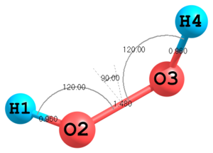 Figure 1. Molecular structure of H2O2.
H
O  1  0.960
O  2  1.480  1  120.0
H  3  0.960  2  120.0  1  120.0
This is a simplest example. First three atoms are defined in a special way, the fourth one is defined in a general way. To specify the first atom no parameters are required, position of the second atom is determined by the H—O bond length, position of the third atom is determined by the O—O bond length and the H—O—O angle. The fourth atom is determined by a triple of parameters: a bond length, an angle and a torsional angle. The values of all parameters are given explicitly in the Z-matrix body. However, in many cases it is more convenient to define variables in a second part of Z-matrix and use them in the first part:
H
O  1  Roh
O  2  Roo  1  Aooh
H  3  Roh  2  Aooh  1  Fhh

Roh=0.960     1
Roo=1.480     1
Aooh=120.0    2
Fhh=120.0     3
In this example it is also demonstrated how group numbers are assigned to parameters. Here two bond lengths
RohandRooare in group1, the angleAoohis in group2and the torsion angleFhhis in group3. The parameters with assigned group numbers can be processed and refined, for example inMINIMIZEprocedure. -
Alternative way for definition of third atom
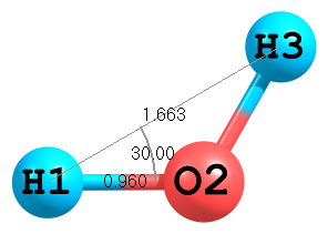 Figure 2. Molecular structure of H2O.
Usually (see first example) position of third atom is determined by a distance to second atom and by an angle to the first atom. Here is an example of an alternative way for definition of the third atom, where a distance to the first atom and an angle of 3—1—2 atoms are used:
H
O  1  Roh
H  1  Rhh  2  Ahho

Roh=0.960
Rhh=1.663
Ahho=30.0
-
Definition of third atom by means of two distances
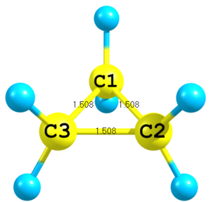 Figure 3. Molecular structure of cyclopropane.
C
C  1  Rcc
C  1  Rcc  2  Rcc     3

Rcc=1.508
Only distances can be used to define position of atoms. For a third atom only two distances are required. Here to define position of the third carbon distances to the first and to the second carbons are used and a special integer key
3is given in the very end of the corresponding line. -
Definition of atoms with distance and two angles
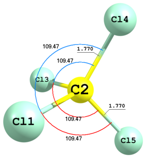 Figure 4. Molecular structure of carbon tetrachloride.
Cl
C    1  R1
Cl   2  R1      1  A1
Cl   2  R1      1  A1      3  A1      -1
Cl   2  R1      1  A1      3  A1       1

     R1          1.7724
     A1        109.47122063
Here is an example of carbon tetrachloride defined with Td symmetry. The last two chlorine atoms are defined using bond lengths and angles, represented as
R1andA1variables. This type of definition is indicated with1or-1keywords in the very end of the corresponding lines. The sign of this keyword always corresponds to the sign of the respective torsion angle X—A—B—C, where X is the defined atom and A, B and C are the first, second and third anchor atoms, respectively. In this example positions of the last two atoms are determined by exactly the same parameters but with two different by sign keys1and-1. -
Definition of atoms using two distances and one angle
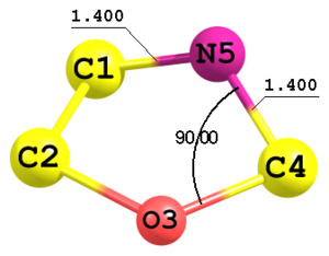 Figure 5. Fragment of a molecule with 5-membered ring.
C
C 1 Rcc
O 2 Rco  1 Acco
C 3 Rco  2 Acoc 1 F1
N 1 Rcn  4 Rcn  3 Anco   2

 Rcc     1.51
 Rco     1.53
 Rcn     1.40
 Acco  106.0
 Acoc  108.0
 Anco   90.0
 F1      0.0
In this example the 5-th atom is defined using two distances C1—N5 and C4—N5 (both equal to
Rcn) and an angle O3—C4—N5 (parameterAnco). This type of definition is indicated by the integer key2in the very end of the line. Sign of this parameter corresponds to the sign of the torsional angle N5—C1—C4—O3. In this case the configuration with parameter-2would be symmetrically equivalent to the presented structure. -
Definition of atoms using two distances and a torsional angle
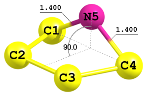 Figure 6. Fragment of another molecule with 5-membered ring.
C
C 1 Rcc
C 2 Rcc2 1 Accc
C 3 Rcc  2 Accc 1 F1
N 1 Rcn  4 Rcn  3 F2  4

 Rcc   1.5152
 Rcc2  1.53
 Rcn   1.40
 Accc  106.0
 F1    0.0
 F2    90.0
This is an example of geometry definition of a five-membered ring in envelope conformation with symmetry Cs. Here the 5-th atom is defined using two distances C1—N5 and C4—N5 (both equal to
Rcn) and a dihedral angle C3—C4—C1—N5 (parameterF2). This is indicated by the key4in the very end of the respective line. There is no-4type since the geometrical configuration is already defined by the sign of the dihedral angle. -
Definition of atoms using three distances
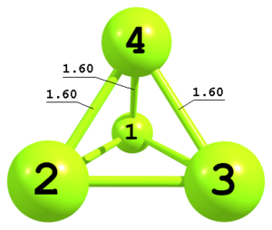 Figure 7. Tetrahedral structure of P4 molecule.
P
P 1 Rpp
P 1 Rpp  2 Rpp           3
P 1 Rpp  2 Rpp  3 Rpp   -3

 Rpp     1.60
This is an example of a Z-matrix for the tetrahedral P4 molecule with only one independent geometrical parameter within Td point group. The third atom is defined as in example 3. The fourth atom is defined using three distances and a key
-3. The sign of the key defines geometrical configuration and corresponds to the sign of the dihedral angle P3—P2—P1—P4. -
Using Cartesian coordinates
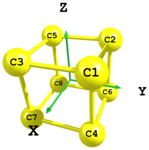 Figure 8. Structure of cubane carbon skeleton.
C   xx   yy   zz
C  -xx   yy   zz
C   xx  -yy   zz
C   xx   yy  -zz
C  -xx  -yy   zz
C  -xx   yy  -zz
C   xx  -yy  -zz
C  -xx  -yy  -zz

 xx = 0.8
 yy = 0.8
 zz = 0.8
In UNEX it is possible to define molecular geometry using Cartesian coordinates within Z-matrix. In this example a cubane carbon skeleton is defined using only Cartesian coordinates. Here formally three independent parameters are used:
xx,yyandzz. However, for the octahedral symmetry they are all equal and can be reduced to just one parameter. Note also the usage of minus signs before variables in some places. -
Mixing Cartesian coordinates and internal parameters
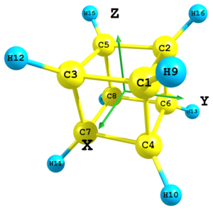 Figure 9. Molecular structure of cubane.
C   xx   yy   zz
C  -xx   yy   zz
C   xx  -yy   zz
C   xx   yy  -zz
C  -xx  -yy   zz
C  -xx   yy  -zz
C   xx  -yy  -zz
C  -xx  -yy  -zz
H 2 Rch 3 Rch 4 Rch  -3
H 1 Rch 6 Rch 7 Rch   3
H 3 Rch 4 Rch 8 Rch   3
H 1 Rch 5 Rch 7 Rch  -3
H 2 Rch 4 Rch 8 Rch  -3
H 5 Rch 6 Rch 7 Rch  -3
H 2 Rch 3 Rch 8 Rch   3
H 1 Rch 5 Rch 6 Rch   3

 xx = 0.8
 yy = 0.8
 zz = 0.8
 Rch = 2.4
In UNEX it is also possible to define molecular geometry using Cartesian and internal coordinates together. The cubane skeleton from the previous example is supplemented here with hydrogen atoms using the ±3 type of definition (three distances). This is only for illustration purposes. In real practice for this molecule in the case of octahedral symmetry it would be more simple to use Cartesian coordinates for definition of hydrogens just like for carbons.
-
Dummy atoms
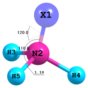 Figure 10. Molecular structure of NH3 with a dummy atom.
X
N 1 1.0
H 2 Rnh  1  Ahnx
H 2 Rnh  1  Ahnx  3   Dx
H 2 Rnh  1  Ahnx  3  -Dx

Rnh=1.1
Ahnx=110.0
Dx=120.0
Dummy atoms can be utilized for definition of molecular structure. The
Xsymbol must be used for them. Also note the possibility to apply negative sign to the dihedral angleDx. -
Centroids
C
H  1 RCH
C  1 RCC 2 120.0
H  3 RCH 1 120.0  2   0.0
C  3 RCC 1 120.0  4 180.0
H  5 RCH 3 120.0  4   0.0
C  5 RCC 3 120.0  6 180.0
H  7 RCH 5 120.0  6   0.0
C  7 RCC 5 120.0  8 180.0
H  9 RCH 7 120.0  8   0.0
C  9 RCC 7 120.0 10 180.0
H 11 RCH 9 120.0 10   0.0
X centroid 1 3 5 7 9 11

RCH=1.08105                1
RCC=1.39157                2
Here the last dummy atom is defined in the centroid of the ring of atoms 1,3,5,7,9 and 11.
-
Explicit numeration of atoms
If default numbering is not acceptable atom numbers can be given explicitly in Z-matrix:
5 X
1 N 5 1.0
2 H 1 Rnh  5  Ahnx
3 H 1 Rnh  5  Ahnx  2   Dx
4 H 1 Rnh  5  Ahnx  2  -Dx

Rnh=1.1
Ahnx=110.0
Dx=120.0
Here the first defined dummy atom is in fact the 5-th in the list of atoms.
-
Definition of atom masses
By default UNEX uses masses of the most stable isotopes of atoms. However, masses of individual atoms can be defined right in Z-matrix, like in the example for D2O below
H 2.0141
O         1 Roh
H 2.0141  2 Roh 1 Ahoh

Roh=1.0
Ahoh=109.0
-
Definition of standard deviations
In UNEX there is a possibility to define values of Z-matrix parameters together with their respective standard deviations. This can be useful if you want to calculate propagation of the defined specific errors to some other dependent geometrical parameters. In the example below the distance
Rnhhas the value1.1and standard deviation0.001, the angleAhnxis defined to be110.0degrees with standard deviation0.2, while the parameterDxis defined with a standard deviation equal to0.0. For the latter it is also possible just to omit the value0.0. Note, for calculation of errors for other dependent geometrical parameters it is necessary to assign group numbers to parameters in Z-matrix, otherwise they will not participate in calculation even if their standard deviations are not zero.X N 1 1.0 H 2 Rnh 1 Ahnx H 2 Rnh 1 Ahnx 3 Dx H 2 Rnh 1 Ahnx 3 -Dx Rnh=1.1 0.001 1 Ahnx=110.0 0.2 2 Dx=120.0 0.0
After definition of Z-matrix it is possible to modify its parameters.
For this purpose SET commands can be used. The example below demonstrates their usage:
SET=BOND,mol, 2,3, 1.3
SET=ANGLE,mol, 1,2,3, 90.0
SET=TORSION,mol, 1,2,3,4, 180.0
Here the first command changes the value of a parameter in a Z-matrix, which corresponds to the distance between atoms 2 and 3. The value of this parameter will be set to 1.3 Å. Analogously, the other two commands set parameters corresponding to the angle 1—2—3 and the torsion angle 1—2—3—4 equal to 90 and 180 degrees, respectively.
Cartesian coordinates
In some cases to perform required computations it is sufficient to define
molecular structure only in form of Cartesian coordinates.
For this purpose MOLXYZ command can be used:
MOLXYZ=mol,format,otag,ctag
Here mol is the name of molecule, format must be one of XYZUNEX, XYZGAUSSIAN or ORCAVPT2, otag and ctag are opening and closing tags of the corresponding data field to be read.
XYZUNEX is a flexible format. In the most complete form each line defines atom number, atom symbol, mass (in amu) and Cartesian coordinates:
<xyz>
1 O  16.0     0.000000    0.000000    0.115719
2 H   1.0     0.000000    0.748790   -0.462876
3 H   1.0     0.000000   -0.748790   -0.462876
</xyz>
Numeration must not be sequentially ordered. The following is also possible:
<xyz>
3 H   1.0     0.000000   -0.748790   -0.462876
1 O  16.0     0.000000    0.000000    0.115719
2 H   1.0     0.000000    0.748790   -0.462876
</xyz>
In the simplest form, numeration and masses can be omitted. In this case sequentially ordered numeration and default masses are assumed.
|
If masses are not given in the data field explicitly and the structure has been already defined earlier, then the original masses are not redefined. |
Default units for Cartesian coordinates are Angstroms. With Units keyword also Bohrs can be used:
<xyz>
Units=Bohr
O           0.00000000     0.00000000     0.12236619
H           0.00000000     1.41500832    -0.97102012
H           0.00000000    -1.41500832    -0.97102012
</xyz>
The other possible format is XYZGAUSSIAN. In can be used for data printed by Gaussian [14] program, for example
<xyz2>
      1          1           0        0.000000    0.000000    1.539305
      2          6           0        0.000000    0.000000    0.458150
      3         17           0        0.000000    1.678636   -0.084082
      4         17           0        1.453741   -0.839318   -0.084082
      5         17           0       -1.453741   -0.839318   -0.084082
</xyz2>
Note, Gaussian can print Cartesian coordinates with or without atomic types (zeros in the example above). Both cases are recognized by UNEX automatically, so the following data can be read using exactly the same command:
<xyz2>
      1          1                    0.000000    0.000000    1.539305
      2          6                    0.000000    0.000000    0.458150
      3         17                    0.000000    1.678636   -0.084082
      4         17                    1.453741   -0.839318   -0.084082
      5         17                   -1.453741   -0.839318   -0.084082
</xyz2>
The other format option is ORCAVPT2.
In this format Orca program [15] prints Cartesian coordinates in VPT2 output files (not the general log file),
for example:
# Atomic coordinates in Angstroem
3
O     8    15.994914620      0.00000000000     -0.06428314752      0.00000000000
H     1     1.007825032      0.75034709185      0.51011010004      0.00000000000
H     1     1.007825032     -0.75034709185      0.51011010004      0.00000000000
Accordingly, UNEX can read the coordinates from the correspodning file using a command like
MOLXYZ=mol,ORCAVPT2,mol.vpt2
or by placing the data directly into UNEX input file between some tags.
Note, UNEX can recognize this format if the string # Atomic coordinates in Angstroem is found.
Upon reading of data the atoms can be automatically renumbered using RENUM command,
which must be given inside the data field:
<xyz1>
RENUM=1-2,2-3,3-1
 C  12.0               -1.03693735   -0.02315941    0.76526551
 C  12.0                0.02512688   -1.12502827    0.77820594
 C  12.0                0.02512688   -1.12502827   -0.77820594
</xyz1>
Here the renumbering works as C1→C2, C2→C3 and C3→C1.
|
|
Potential functions
|
Starting from UNEX 1.6-990 the input numeration of parameters for potential functions starts from zero! |
In order to construct a dynamic model for molecular part of electron diffraction intensity
a potential function must be introduced.
This can be done using POTENTIAL command:
POTENTIAL=mol,format,otag,ctag
here mol is the name of molecule, format can be PTL1 or FUNC, otag and ctag are
opening and closing tags of data field as usually.
The PTL1 format is for the case when potential function is introduced in numerical form, for example
POTENTIAL=mol,PTL1,<pot>,</pot>

<pot>
  0.0  52.759317
 10.0  52.265898
 20.0  50.701285
 30.0  47.791786
 40.0  43.252047
 50.0  37.535062
 60.0  31.751394
 70.0  23.594173
 80.0  13.194505
 90.0   5.294997
100.0   1.090070
110.0   0.000000
</pot>
Here in the first column are the values of the geometric parameter corresponding to the dynamic coordinate
In the second column are the respective energy values; their units can be defined by PotEUnits keyword in BASE.
After reading the data UNEX performs two major actions.
First, all the values are shifted so the the minimal value equals to zero.
Second, the data are approximated with a function.
Type of the function depends on the PotType setting in the field of the respective molecule.
If it is a parametric function then the PotCoefNum keyword should be set to a proper value.
Note, this keyword defines total number of parameters in the potential function including free term, if applicable.
For example, the combination PotType=Cos1 and PotCoefNum=3 defines the following potential function
(note the numeration of parameters Vi):
![$$V = V_0 + \frac {V_1}{2} \left[ 1 - \cos(1 \times F) \right] + \frac {V_2}{2} \left[ 1 - \cos(2 \times F) \right]$$](images/stem-7a3fae8cd12b37c2a66cfc9883a9463b.svg)
Similarly, for PotType=Polynom and PotCoefNum=5 the potential function will be

The model Gauss for potential function has no free term and the combination PotType=Gauss and PotCoefNum=6 gives

Data field in PTL1 format may contain two special keywords: POTCOEFV and POTCOEFG.
The first one is for setting initial values for parameters of model potential function.
They are used in approximation procedure.
Generally, for cosine series they are not required but for a sum of gaussians it is very advisable
to set them to some reasonable values, which will be refined further by UNEX.
The other keyword, POTCOEFG, is for setting group numbers for those parameters,
which should be refined in MINIMIZE and related commands.
The example below demonstrates both keywords
<pot>
POTCOEFG=0-31,1-32,2-33,3-34,4-35,5-36
POTCOEFV=0-53.0,1--0.3,2-1.0,3-2.0,4--2.8,5-1.0
        0.0    -2104.2041440921
      -10.0    -2104.2043320255
      -20.0    -2104.2049279551
      -30.0    -2104.2060361246
      -40.0    -2104.2077652201
      -50.0    -2104.2099427046
      -60.0    -2104.2121455875
      -70.0    -2104.2152525088
      -80.0    -2104.2192135333
      -90.0    -2104.2222222971
     -100.0    -2104.2238238691
     -110.0    -2104.2242390548
     -120.0    -2104.2240176886
     -130.0    -2104.2236761259
     -140.0    -2104.2234703951
     -150.0    -2104.2234587732
     -160.0    -2104.2235955815
     -170.0    -2104.2237665581
     -180.0    -2104.2238429817
</pot>
Several important points can be mentioned for this example.
-
The energy values are given in atomic units so
PotEUnits=aushould be defined in BASE. -
This potential is best described with a sum of two gaussians, so
PotType=Gaussshould be defined in molecular data field. -
Two gaussians require in total six parameters, so
PotCoefNum=6should be defined. -
POTCOEFGdefines group numbers for potential function parameters in formatParameterNumber-GroupNumber. In this example the parameters get group numbers 31—36. -
POTCOEFVdefines initial values for potential function parameters in formatParameterNumber-Value. For negative values the format includes the second minus signParameterNumber--Value. In this example the initial values for parameters are 53.0 for V1, -0.3 for Δ1, 1.0 for w1, 2.0 for V2, -2.8 for Δ2 and 1.0 for w2. See above for the example of analytical expression of the sum of two gaussians. -
Numeration of parameters in
POTCOEFGandPOTCOEFVstarts from zero. -
Not necessarily all parameters should be declared in
POTCOEFGandPOTCOEFV.
|
With a |
The other available format FUNC is for the case of introducing particular values of parameters for the potential function.
The following example demonstrates the usage of this format.
POTENTIAL=mol,FUNC,<pot>,</pot>

<pot>
0 0.0
1 1.5    101
2 0.2    102
3 0.001
4 0.04   103
</pot>
In the data field at least two columns must be defined. The first column is for parameter indices,
the second column contains values of respective parameters.
The optional third column can contain group numbers for respective parameters.
In this example the introduction of values for first five parameters is done.
As in the examples above the keys PotType and PotCoefNum here also should be defined before reading the data.
Additionally, group numbers 101, 102 and 103 are assigned to parameters 1, 2 and 4, respectively.
Note, the numeration of parameters starts from zero. The scheme for numeration is as described above.
For Gauss models special scheme is used: the parameters 0, 1 and 2 correspond to V, Δ, and w of the first Gaussian in the sum.
The next tripple, 3, 4 and 5, correspond to parameters V2, Δ2 and w2 (parameters of the second Gaussian) and so on.
It is possible to execute several POTENTIAL commands with FUNC format introducing different values
of parameters and/or group numbers if required.
Also it is not necessary to set all parameters in the data field. It is possible to define values only for selected parameters.
In this case the other parameters will not be affected.
|
There is no general scheme for units of parameters for all types of parametric potential functions. Thus UNEX reads values of parameters without any internal conversion. It is user’s responsibility to define values so that potential function gives energy in kJ/mol for dynamic coordinate in radians. |
Vibrational data
Quadratic force constants
Quadratic (also known as harmonic) force constants in Cartesian coordinates are introduced with the F2C command:
F2C=mol,format,otag,ctag
Reading of data can be done in several formats: FREEFC, GAUSSIANARCH, CFOURFCM, CFOURLOG, CFOURFJA64 and ORCAHESS.
The option FREEFC is used when data are not formatted in any particular manner.
UNEX reads floating point numbers line by line from left to right and correspondingly fills
the lower-left triangle of force constants matrix.
The data must be provided in Hartree Bohr-2 units.
For example, data for a triatomic molecule can look like
F2C=mol,FREEFC,<data2>,</data2>

<data2>
-0.00011
 0.00000  0.69921
 0.00000  0.00000  0.47159
 0.00006  0.00000  0.00000 -0.00006
 0.00000 -0.34961  0.20819  0.00000  0.38113
 0.00000  0.27346 -0.23580  0.00000 -0.24082  0.22485
 0.00006  0.00000  0.00000  0.00001  0.00000  0.00000 -0.00006
 0.00000 -0.34961 -0.20819  0.00000 -0.03153 -0.03264  0.00000  0.38113
 0.00000 -0.27346 -0.23580  0.00000  0.03264  0.01095  0.00000  0.24082  0.22485
</data2>
or
F2C=mol,FREEFC,<data3>,</data3>

<data3>
  -0.00011233   0.00000000   0.69921020   0.00000000   0.00000000
   0.47159438   0.00005616   0.00000000   0.00000000  -0.00006270
   0.00000000  -0.34960510   0.20818553   0.00000000   0.38113336
   0.00000000   0.27346025  -0.23579719   0.00000000  -0.24082289
   0.22485174   0.00005616   0.00000000   0.00000000   0.00000654
   0.00000000   0.00000000  -0.00006270   0.00000000  -0.34960510
  -0.20818553   0.00000000  -0.03152826  -0.03263736   0.00000000
   0.38113336   0.00000000  -0.27346025  -0.23579719   0.00000000
   0.03263736   0.01094545   0.00000000   0.24082289   0.22485174
</data3>
GAUSSIANARCH is the format of archive entry in the very end of Gaussian [14] output files.
Here is an example for water molecule (a part of Gaussian output obtained from a calculation with Freq keyword):
F2C=mol,GAUSSIANARCH,<data>,</data>

<data>
 1\1\GINC-CHEOPS10401\Freq\RPBE1PBE\6-31G(d,p)\H2O1\YVISHNEV\04-Nov-201
 5\0\\#P PBE1PBE/6-31G(d,p) Freq\\H2O\\0,1\O,0.,0.,0.118417\H,0.,0.7569
 23,-0.473669\H,0.,-0.756923,-0.473669\\Version=EM64L-G09RevD.01\State=
 1-A1\HF=-76.3369645\RMSD=8.979e-09\RMSF=4.171e-06\ZeroPoint=0.0217171\
 Thermal=0.024552\Dipole=0.,0.,-0.8151838\DipoleDeriv=-0.7285751,0.,0.,
 0.,-0.4461319,0.,0.,0.,-0.3542551,0.3642876,0.,0.,0.,0.223066,0.078652
 ,0.,0.1104485,0.1771276,0.3642876,0.,0.,0.,0.223066,-0.078652,0.,-0.11
 04485,0.1771276\Polar=3.0234315,0.,7.2833047,0.,0.,5.4419574\PG=C02V [
 C2(O1),SGV(H2)]\NImag=0\\-0.00011233,0.,0.69921020,0.,0.,0.47159438,0.
 00005616,0.,0.,-0.00006270,0.,-0.34960510,0.20818553,0.,0.38113336,0.,
 0.27346025,-0.23579719,0.,-0.24082289,0.22485174,0.00005616,0.,0.,0.00
 000654,0.,0.,-0.00006270,0.,-0.34960510,-0.20818553,0.,-0.03152826,-0.
 03263736,0.,0.38113336,0.,-0.27346025,-0.23579719,0.,0.03263736,0.0109
 4545,0.,0.24082289,0.22485174\\0.,0.,-0.00000976,0.,0.00000261,0.00000
 488,0.,-0.00000261,0.00000488\\\@
</data>
|
Instead of copying data to UNEX input file it is also possible to read the data directly from other files. For this, after the format only the name (with path, if reqired) of the file with the data must be provided as F2C=mol,GAUSSIANARCH,calculation.log This option is available for |
In the case of GAUSSIANARCH format there is a possibility to define which particular archive entry will be parsed by UNEX.
For this, the keyword Entry must be used. For example, if you have a multi-job Gaussian output file and want to read the
data from the second archive entry, then you must use
F2C=mol,GAUSSIANARCH,calculation.log Entry=2
Otherwise by default only the first entry is be parsed and processed.
The format CFOURFCM is used for reading force constants as they are written by the Cfour program [16] in FCM files,
for example
F2C=mol,CFOURFCM,<data1>,</data1>

<data1>
2   12
   -0.0000000000        0.0000000000        0.0000000000
    0.0000000000        0.0000000000        0.0000000000
    0.0000000000       -0.0000000000        0.0000000000
    0.0000000000        0.0000000000        0.0000000000
    0.0000000000        0.0000000000        2.0658524394
    0.0000000000        0.0000000000       -2.0658524394
    0.0000000000        0.0000000000        0.0000000000
   -0.0000000000        0.0000000000        0.0000000000
    0.0000000000        0.0000000000        0.0000000000
    0.0000000000       -0.0000000000        0.0000000000
    0.0000000000        0.0000000000       -2.0658524394
    0.0000000000        0.0000000000        2.0658524394
</data1>
Note, in this format Cfour prints full matrix of force constants and UNEX reads all the data.
The other format option CFOURLOG is used for reading harmonic force constants from Cfour log files.
The respective data may look like
           CL#1 x      CL#1 y      CL#1 z      CL#2 x      CL#2 y      CL#2 z

 CL#1 x    0.037440
 CL#1 y    0.000000    0.150729
 CL#1 z    0.000000   -0.080107    0.094084

 CL#2 x    0.005503    0.000000    0.000000    0.037440
 CL#2 y    0.000000   -0.042209   -0.004598    0.000000    0.150729
 CL#2 z    0.000000    0.004598    0.007082    0.000000    0.080107    0.094084
|
It is important to check the molecular orientation, for which the Hessian is printed in Cfour log. Also, the numeration of atoms in the Hessian can be different from that in input file! |
CFOURFJA64 option is suitable for Cfour formatted job archive files (FJOBARC), which are produced by the Cfour program using 64 bit integers.
In this format the data starts with the string D2EZORDR, for example (only few lines are shown):
D2EZORDR
    -1619558400     1052094016              0              0
              0              0    -1800863744    -1096438098
              0              0              0              0
    -1800863744    -1096438098              0              0
              0              0              0              0
    -1541880946     1072243206              0              0
              0              0    -1542781662    -1076289018
      961544973     1070820251              0              0
    -1542781662    -1076289018      961544973    -1076663397
              0              0              0              0
Using the ORCAHESS format it is possible to read force constants in Cartesian coordinates as they are printed by Orca [15]
program in *.hess files after the keyword $hessian, for example (only first few lines are shown here):
$hessian
9
                    0                  1                  2                  3                  4
    0      8.0292682091E-01   8.3460223548E-14   9.7340153014E-17  -4.0146341046E-01  -3.0732160356E-01
    1      8.3460223548E-14   5.4244904491E-01  -1.9508314770E-16  -2.4246471749E-01  -2.7122452246E-01
    2      9.7340153014E-17  -1.9508314770E-16   2.5021344996E-09   1.2784996001E-16   9.5383934231E-17
Cubic force constants
Cubic force constants in Cartesian coordinates are introduced with the F3C command:
F3C=mol,format,otag,ctag
In this case the only available format is GAUSSIANARCH, which expects Gaussian archive entry with cubic force constants
in Cartesian coordinates, printed in jobs with the Freq=cubic keyword. Note, you can control from which entry to read the data
using the Entry keyword in the same way as for the F2C command (see above).
Cubic force constants in normal coordinates can be read into UNEX with the F3N command:
F3N=mol,format,otag,ctag
The available format is IDXLIST, which is the list of indices with respective force constant one per line, for example:
F3N=mol,IDXLIST,<cubic>,</cubic>

<cubic>
Units=cm
    7    7    7           311.3047211506
    7    7    8           338.7184194394
    7    8    8           -38.5261283132
    8    8    8         -1848.3145392607
    7    9    9          -246.5539755370
    8    9    9         -1854.0526848303
</cubic>
Here the first three integers are indices (i, j, k) of normal modes, the numbering starts from 1, first 6 (5) modes correspond to rotations and translations.
After the indices the corresponding force constant is given. Note, in this example the units for the constants are explicitly defined with the Units keyword.
It has two options, Hartree-amu-Bohr (corresponds to units Hartree amu-3/2 Bohr-3, this is assumed by default) and cm (means reduced values in cm-1).
The units can also be defined in the command line. For example, to read in data in cm-1 from the external file cubic.dat one can do
F3N=mol,IDXLIST,cubic.dat Units=cm
Note, UNEX assumes force constants equal to zero for combinations (i, j, k) not given in the input. Also, in this mode it makes no sence to provide on input multiple equivalent (i, j, k), for example both (7, 8, 9) and (7, 9, 8), as they correspond to the same value of the force constant due to symmetry properties. The last readed value will be used by UNEX.
Vibrational modes
In UNEX there is a command VMOD, which can be used both for reading in and for processing of data related to vibrational modes.
Input modes are described here, for the details on processing see the section Vibrational analysis.
If it is required only to input frequencies, then the following variant of the command can be used:
VMOD=mol,READFREQ,otag,ctag
For example, reading frequencies (in cm-1) for water can be done simply as:
VMOD=h2o,READFREQ,<freq>,</freq>
<freq>
1737.01
3988.50
4145.43
</freq>
Vibrational modes can be scaled (multiplied by a factor). Scale factors for each mode defined in mass-weighted Cartesian coodinates are introduced by the command
VMOD=mol,READSCALEMC,<modsc>,</modsc>
where the respective data looks like
<modsc>
7 -1.0
8 -1.0
9 -1.0
</modsc>
In this example the scale factors (each equal to -1) are given for vibrational modes 7, 8 and 9. Notice, the first six (five for linear molecules) modes correspond to translations and rotations. So the numbering for vibrational modes starts from 7 (6 for linear molecules).
Complete vibrational modes can be read directly. For this UNEX supports two formats: ORCAHESS and CFOURFJA64.
Using the ORCAHESS format it is possible to read the modes appearing in Orca *.hess files after the keyword $normal_modes
VMOD=mol,ORCAHESS,h2o_orca.hess
The respective part of the h2o_orca.hess file may look like
$normal_modes
9 9
                    0                  1                  2                  3                  4
    0      0.0000000000E+00   0.0000000000E+00   0.0000000000E+00   0.0000000000E+00   0.0000000000E+00
    1      0.0000000000E+00   0.0000000000E+00   0.0000000000E+00   0.0000000000E+00   0.0000000000E+00
    2      0.0000000000E+00   0.0000000000E+00   0.0000000000E+00   0.0000000000E+00   0.0000000000E+00
    3      0.0000000000E+00   0.0000000000E+00   0.0000000000E+00   0.0000000000E+00   0.0000000000E+00
    4      0.0000000000E+00   0.0000000000E+00   0.0000000000E+00   0.0000000000E+00   0.0000000000E+00
    5      0.0000000000E+00   0.0000000000E+00   0.0000000000E+00   0.0000000000E+00   0.0000000000E+00
    6      0.0000000000E+00   0.0000000000E+00   0.0000000000E+00   0.0000000000E+00   0.0000000000E+00
    7      0.0000000000E+00   0.0000000000E+00   0.0000000000E+00   0.0000000000E+00   0.0000000000E+00
    8      0.0000000000E+00   0.0000000000E+00   0.0000000000E+00   0.0000000000E+00   0.0000000000E+00
                    5                  6                  7                  8
     0      0.0000000000E+00   2.1663493053E-17  -2.6137484626E-17   7.0336524903E-02
     1      0.0000000000E+00   7.0212439058E-02  -5.0516880408E-02  -3.0959555454E-17
     2      0.0000000000E+00  -2.6011329560E-18   7.1419641812E-18  -1.0336224485E-17
     3      0.0000000000E+00   4.3256186384E-01   5.8140271968E-01  -5.5814293360E-01
     4      0.0000000000E+00  -5.5715827254E-01   4.0086768384E-01  -4.3128047986E-01
     5      0.0000000000E+00   1.0703631299E-16  -1.2062467606E-16   2.0674220999E-16
     6      0.0000000000E+00  -4.3256186384E-01  -5.8140271968E-01  -5.5814293360E-01
     7      0.0000000000E+00  -5.5715827254E-01   4.0086768384E-01   4.3128047986E-01
     8      0.0000000000E+00  -6.5754660800E-17   7.2771131778E-18  -4.2699682611E-17
Normal modes can be read from Cfour formatted job archive files (FJOBARC), if they are created by a 64-bit integer version of Cfour.
For this, the CFOURFJA64 format must be used. The data in this format starts from the string NORMCORD followed by list of signed integers.
Here is an example (with shortened data field):
VMOD=mol,CFOURFJA64,<ncoord>,</ncoord>
<ncoord>
NORMCORD
     -866626241     1070475579    -1492162202    -1098255852
     1998126717    -1096612452    -1408212297     1070475562
      341220828    -1098255824     1455666656    -1096612443
    -1406332546     1070475562      342250045    -1098255824
    -1754433024    -1096612461     1288255770    -1096613896
</ncoord>
Naturally, you must not necessarily copy the data to the UNEX input file.
Instead, the name of the file with the data can be indicated in the VMOD command:
VMOD=mol,CFOURFJA64,FJOBARC
ED terms
A term in GED is a pair of atoms with associated parameters like distance, vibrational amplitude, correction and asymmetry (anharmonic, phase-shift) constant.
Vibrational amplitudes, corrections and asymmetry constants required for calculation of ED molecular intensities can be introduced with AMPLITUDES command.
The syntax of the command is as usual:
AMPLITUDES=mol,format,otag,ctag
where format can be either FREEU, SHRINKU or ELDIFF.
An example of data field in FREEU format:
<ampl>
#a1  a2     comment       l        corr         a       g
#
O1   H2     0.9591      0.0675   -0.0126     2.0000     1
O1   H3     0.9591      0.0675   -0.0126     2.0000     1
H2   H3     1.5063      0.1125   -0.0129     1.0000     2
</ampl>
Here each line includes a pair of atoms, arbitrary comment (here the distance between atoms is used as a comment),
amplitude l, vibrational correction corr, asymmetry constant a and group number g.
Amplitudes and corrections must be given in Å.
By default the type and units for asymmetry constants depend on the current setting of the ImolAnhTermModel keyword (for details see see chapter Models for ED intensity).
For ImolAnhTermModel=Asym the default expected type is here asymmetry parameter κ and the expected units are Å3.
In case of ImolAnhTermModel=Morse the expected type is Morse parameter and the units are Å-1.
However, it is possible to define explicitly the type and units for the input a-parameters with the local keyword a-Units as in the example:
<ampl>
a-Units=kA3
O1   H2     0.9591      0.0675   -0.0135     8.0e-6
O1   H3     0.9591      0.0675   -0.0135     8.0e-6
H2   H3     1.5063      0.1125   -0.0137     1.8e-6
</ampl>
The setting kA3 for a-Units indicates here that the input a-values are in fact asymmetry constants κ in Å3.
If the global keyword ImolAnhTermModel is set to Morse, then these values are converted internally to Morse constants
according to the formula

where l is the respective amplitude taken from the same current input. Another option is kpm3 if κ are given in pm3.
Yet another option is a-Units=c3pm3, indicating that the input values are c3 parameters from the cumulant approximation [17].
They are converted internally to asymmetry parameters as κ = 10-6c3/6.
Again, if ImolAnhTermModel=Morse, than Morse constants are calculated automatically as described above.
Also it is possible to indicate explicitly the input of Morse constants in Å-1 by defining a-Units=MoAm1.
If at this point the current setting is ImolAnhTermModel=Asym, then the input Morse constants are automatically recalculated
into asymmetry parameters κ according to the formula above.
Group numbers g may be defined for amplitudes. However, if you do not need to assign group numbers (no need to refine amplitudes), there is no need to set them to zeros explicitly. Instead, they may be simply omitted
<ampl>
#At1 At2   comment       l        corr         a       g
#
O1   H2     0.9591      0.0675   -0.0126     2.0000
O1   H3     0.9591      0.0675   -0.0126     2.0000
H2   H3     1.5063      0.1125   -0.0129     1.0000
</ampl>
If a-parameters are zero, they also can be omitted. Note, group numbers may still be defined
<ampl>
#At1 At2    comment       l        corr         a       g
#
O1   H2     0.9591      0.0675   -0.0126                1
O1   H3     0.9591      0.0675   -0.0126                1
H2   H3     1.5063      0.1125   -0.0129
</ampl>
If a correction is zero and the respective a-parameter is also zero, then both numbers may be omitted. But if the correction is zero and the a-parameter is not zero, then both numbers must be defined explicitly.
<ampl>
#At1 At2    comment       l        corr         a       g
#
O1   H2     0.9591      0.0675
O1   H3     0.9591      0.0675                          1
H2   H3     1.5063      0.1125    0.0000     1.0000
</ampl>
Another format option is SHRINKU. It is implemented for reading data produced by the Shrink [18] program.
Specifically UNEX expects data as it is printed by Shrink in tables for the second approximation:
<ampl>
#Amplitudes and corrections at 0010 K, second (harmonic)
#approximation, local centrifugal distortions included;
#<dr()> are deviations from equilibrium distances
#
#   Atoms   Distance  Amplitude <dr(loc)> <dr(har)>      K
#
1  O1   H2   0.9591     0.0675    0.0011    0.0000    0.00365    1
2  O1   H3   0.9591     0.0675    0.0011    0.0000    0.00365    2
3  H2   H3   1.5063     0.1125    0.0001   -0.0038    0.01201    3
</ampl>
From the given data UNEX reads amplitudes (from the fifth column) and corrections
(Shrink prints them in the column K, in the second approximation they correspond to rh1-ra).
The values in columns <dr(loc)> and <dr(har)> are ignored.
Note, in Shrink output the integers in the last column are simply indices of the corresponding atom pairs.
In contrast, UNEX interprets them as group numbers. In reality it is very unlikely that one would leave them as they are.
Normally you need to delete this column and assign group numbers manually or in another way, as needed.
If you want to use anharmonic corrections from Shrink, the column K must be substituted with the column r_e-r_a
from the very last table produced by Shrink, so the format remains for UNEX unchanged.
In the example below corrections to equilibrium structure are used and the integers are removed as it is normally done.
<ampl>
1  O1   H2   0.9591     0.0675    0.0011    0.0000   -0.0126
2  O1   H3   0.9591     0.0675    0.0011    0.0000   -0.0126
3  H2   H3   1.5063     0.1125    0.0001   -0.0038   -0.0129
</ampl>
The third available format ELDIFF is for introducing data produced by the ElDiff [19] program.
Here is a shortened example of such data field:
<ampl>
#At.pair  Num    Re     Rg     Ra     Dr    Dr(har) Dr(kin) Dr(dyn) Ampl.  c3/6
Cl1-C2   ( 1) 1.7609 1.7687 1.7672  0.0078 0.0027  0.0009  0.0042 0.0517   2.59 555
Cl1-Cl3  ( 1) 2.8755 2.8857 2.8841  0.0102 0.0018 -0.0017  0.0101 0.0668   3.76
</ampl>
Vibrational corrections are calculated from the input data as differences Re-Ra.
Amplitudes and asymmetry parameters c3/6 are read as they are given.
Note, the input c3/6 values in pm3 are converted internally to asymmetry parameters κ in Å3.
However, they can be internally further converted to Morse parameters if the ImolAnhTermModel keyword is set to Morse.
As usually, optional integers in the very end of lines are the group numbers for
refinements of the respective amplitudes or their scale factors.
If due to some reason the numeration of atoms in the input data does not coincide with already defined numeration
(for example, in Z-matrix), the RENUM command can be used:
<ampl>
RENUM=1-2,2-3,3-1
1  O1   H2   0.9591     0.0675    0.0011    0.0000   -0.0126
2  O1   H3   0.9591     0.0675    0.0011    0.0000   -0.0126
3  H2   H3   1.5063     0.1125    0.0001   -0.0038   -0.0129
</ampl>
It works in the same way as in the case of reading Cartesian coordinates.
Namely, in the example above the following numeration will be done: O1→O2, H2→H3 and H3→H1.
RENUM works in fields of all format types.
Note, multiple RENUM commands can be defined in the same data field and UNEX will process all of them.
This can be useful when large amount of atoms must be renumbered and the corresponding list would be too long for a single RENUM command.
As already mentioned integer numbers in the very end of lines are interpreted by UNEX as group numbers for amplitudes so that they can be refined.
In case of dynamic GED models group numbers can be defined only for the first pseudoconformer in the psconfs list (see above).
Group numbers for amplitudes of other pseudoconformers are assigned automatically and coincide with those for the first pseudoconformer.
In general AMPLITUDES allows introducing vibrational amplitudes, corrections,
asymmetry constants and group numbers for amplitudes. It is not guaranteed that
with this command interatomic distances can be introduced.
Another limitation is the imposibility to define group numbers for ra distances,
when there is a need to refine them as independent parameters.
Thus the AMPLITUDES command is used mostly for geometrically consistent models,
when molecular structures are defined in terms of Z-matrices or Cartesian coordinates.
There is, however, an alternative command GEDTERMS for defining all required parameters
for calculation of ED molecular intensity curves
GEDTERMS=mol,GTRM,otag,ctag
It accepts only one type of format GTRM, which assumes that each line contains a pair of atoms,
ra distance, amplitude, correction (normally zero), asymmetry constant and group numbers for the distances and amplitudes
as shown in the example below
<gtrm>
#At1 At2      r_a         l        corr         a       Gr     Gl
#
C2   Cl1    1.7625     0.05485     0.00      0.00001     3      5
C2   Cl3    1.7625     0.05485     0.00      0.00001     3      5
C2   Cl4    1.7625     0.05485     0.00      0.00001     3      5
C2   Cl5    1.7625     0.05485     0.00      0.00001     3      5
Cl1  Cl3    2.8871     0.06844     0.00      0.00002     4      6
Cl1  Cl4    2.8871     0.06844     0.00      0.00002     4      6
Cl1  Cl5    2.8871     0.06844     0.00      0.00002     4      6
Cl3  Cl4    2.8871     0.06844     0.00      0.00002     4      6
Cl3  Cl5    2.8871     0.06844     0.00      0.00002     4      6
Cl4  Cl5    2.8871     0.06844     0.00      0.00002     4      6
</gtrm>
Note, the definition of a-parameters follows here the same rules as for the AMPLITUDES command,
likewise it is possible to use the local RENUM command and the a-Units keyword. See above for details.
For investigation purposes with UNEX it is possible to refine ra distances independently,
resulting in a so-called geometrically inconsistent structure.
The corresponding group numbers for ra distances can be defined only with the GEDTERMS command.
|
Both |
|
UNEX can automatically check values of parameters for symmetrically equivalent terms.
This is done if symmetry has been determined for the molecule before introducing parameters for terms, for example by calling |
It is possible to set all distance corrections of a molecule to a single value at once.
For this the SET command can be used as SET=ALLRCORR,mol,value. For example,
SET=ALLRCORR,mymol 0.0
will zero out all distance corrections in the mymol molecule.
ED scattering factors
For calculation of theoretical molecular contribution to the total electron diffraction intensity scattering factors are required. In chapter Models for ED intensity these factors are denoted as f-functions, which characterize scattering ability of atom pairs. Also in some cases it is convenient to operate with so called g-functions defined as the ratio

where Iat is the atomic contribution to the total electron scattering intensity.
In UNEX calculation of all these functions can be done using the GF command:
GF=mol,AUTO,<electron_energy> Units=[A,kV]
where <electron_energy> is the floating point number defining the energy of electrons.
There are two possibilities to provide this quantity, in form of the electron wavelength in (in Å)
or using accelerating voltage (in kV). This is controlled by the optional keyword Units,
which accepts options A for Angstroms and kV for kilovolts.
The electron wavelength and accelerating voltage are recomputed in each other internally in UNEX
using the formula (4.3.1.33) in [8].
By default the electron wavelength is expected, so for example the command
GF=mol,AUTO,0.05
calculates scattering factors for mol and the electron wavelength 0.05 Å.
This is equivalent to the command
GF=mol,AUTO,56.9871878 Units=kV
The methods for calculation of elastic and inelastic scattering factors are globally defined using the keywords EDElScatFacMethod and EDInelScatFacMethod, respectively.
For electrons with energy 10-100 kV the options PwTab2 and MorseTab2 are recommended.
In this case UNEX uses built-in tables [8] of inelastic factors and scattering aplitudes and phases defined for the accelerating voltages 10, 40, 60, 90 kV and for s-values up to 60 Å-1.
Two-dimensional cubic splines are used for calculation of required parameters from tabulated values.
Note, for accelerating voltages outside the 10-90 kV range the scattering aplitudes and phases are calculated by cubic extrapolation.
This may be inaccurate for energies significantly deviating from the stated range.
For MeV electrons the recommended options are Born1Tab1C1 and MorseTab2, respectively.
Note, the GF command can be called multiple times for the same molecule.
The corresponding functions will be recalculated with defined parameters.
ED intensities
UNEX has a special system for referencing of all types of intensity curves.
Each curve is defined as a pair of integer numbers, for example 1-1 represents in the input syntax a particular curve.
This system is designed to simplify categorization of curves and is closely related to the format (see below) of their definition in UNEX input files.
The most common and natural for GED basis for categorization of curves is the distance between nozzle and detector.
There can be, however, other considerations how to form groups of curves, by methods of data reduction and processing, by dates of experiments, this is up to user.
Total intensity
To introduce total intensity curves INT command is used:
INT=READ,otag,ctag
The simplest example of the data field is
<INT>
INT1
 7.4000000000        5.8921150540
 7.6000000000        5.6976865331
 7.8000000000        5.5221522042
 8.0000000000        5.3696527781
 8.2000000000        5.2437855620
 8.4000000000        5.1021824331
 8.6000000000        4.9709462648
 8.8000000000        4.8373286097
 9.0000000000        4.7019566330
 9.2000000000        4.5680270813
 9.4000000000        4.4361494355
 9.6000000000        4.3235065367
 9.8000000000        4.2099473887
10.0000000000        4.1088546902
</INT>
In the first column are s-values, in the second column are values of total electron scattering intensity.
Here only one intensity curve is defined. In UNEX syntax it can be referenced as 1-1 curve.
The input format requires that each data set starts with an INT keyword followed by an integer number.
In the example above it is INT1, which means first group. This is first definition of an INT1 curve, therefore it has the 1-1 reference code.
You can input several data sets in the first group as in the following example
<INT>
INT1
 7.4000000000        5.8921150540
 7.6000000000        5.6976865331
 7.8000000000        5.5221522042
INT1
 9.6000000000        4.3235065367
 9.8000000000        4.2099473887
10.0000000000        4.1088546902
</INT>
Here the first curve from above is 1-1, the second one gets the code 1-2.
In the same way a second and so on groups of intensities can be introduced:
<INT>
INT1
 7.4000000000        5.8921150540
 7.6000000000        5.6976865331
 7.8000000000        5.5221522042
INT1
 9.6000000000        4.3235065367
 9.8000000000        4.2099473887
10.0000000000        4.1088546902
INT2
28.1000000000        1.0475326418
28.2000000000        1.0393546185
28.3000000000        1.0276683596
INT2
28.0000000000        1.0475326418
28.2000000000        1.0393546185
28.3000000000        1.0276683596
30.0550000000        1.0159231825
</INT>
Here curves 1-1, 1-2, 2-1 and 2-2 are defined.
Note, UNEX assumes no constant step on the s-scale. The only requirements are that
-
s and intensity values must be positive,
-
s-values must be sorted in ascending order,
-
there must be no equal s-values, differences smaller than
MinDsare not allowed.
The UNEX input format also allows introducing standard deviations for intensity values:
<INT>
INT1
6.2000000000        7.4146108106        0.0039183246
6.4000000000        7.1488355268        0.0021688941
6.6000000000        6.8938017418        0.0021065446
6.8000000000        6.6412539602        0.0020678461
7.0000000000        6.3619711300        0.0020204005
7.2000000000        6.1273418113        0.0019858103
7.4000000000        5.8921150540        0.0019449769
7.6000000000        5.6976865331        0.0019131756
7.8000000000        5.5221522042        0.0018765991
8.0000000000        5.3696527781        0.0018468983
</INT>
Here as usually in the first and second columns are s and intensity values and in the third column are the respective standard deviations of the intensity values. They can be used by UNEX in different procedures, for example in least-squares refinement method. Standard deviations are optional and can be defined only for particular points:
<INT>
INT1
6.2000000000        7.4146108106
6.4000000000        7.1488355268        2.0
6.6000000000        6.8938017418
6.8000000000        6.6412539602        2.0
</INT>
Here we define standard deviations 2.0 for two points, for the rest default value is assumed. The default value can be defined by using GStdev keyword.
Also note that in this example we define standard deviations for total intensity. However, using respective setting for the keyword TypeStdev (see below) it is possible to define standard deviations for molecular intensity sM(s), which may be later calculated from the input total intensity.
UNEX allows setting special parameters related to particular intensity curves. They are defined after corresponding INT keywords like in the example
<INT>
INT1 Parameter1=value Parameter2=value
6.2000000000        7.4146108106
6.4000000000        7.1488355268
6.6000000000        6.8938017418
6.8000000000        6.6412539602
</INT>
Note, there must be no space characters in pairs Parameter=value.
| The set of parameters, which should be defined for each intensity curve depends on the particular application. Various procedures in UNEX may require different parameters to be defined. |
Possible parameters are
- Scale
-
Scale factor for molecular intensity curve. The default value is 1.0.
- VarSc
-
Group number in
MINIMIZEand alike procedures. If this parameter equals to a positive integer number then the respective scale factor will be refined. - NtoP
-
Nozzle-to-Plate — distance from diffraction point to the detector in mm. Input s-values must correspond to this value.
- NewNtoP
-
New nozzle-to-plate value in mm. Input s-values will be recalculated using defined
NtoPandNewNtoP. - StoP
-
Sector-to-Plate — distance from rotating sector defice to the detector in mm.
- Lam
-
Lambda — electron wavelength in Å. This parameter tells UNEX for which electron wavelength correspond input s-values.
- NewLam
-
New value of electron wavelength in Å. This should be defined together with
Lamif you want to recalculate input s-values for the new value of electron wavelength. - Tfac
-
t-factor — a value proportional to the exposure time in the measurement of the corresponding diffraction pattern. This parameter can be used in models for the total intensity. For description of models see introduction to the theory of background lines.
- Std
-
Set this parameter to
CCl4,C6H6,CS2orCO2if the intensity corresponds to one of these compounds and you want to use it for determination of electron wavelength withSTANDARDcommand. - BglNinflThr
-
Threshold for the number of inflection points on background line. By default the value of this keyword is negative, indicating that the global setting must be used (see keyword
BglNinflThr). - RBPSDThr
-
Threshold for the relative power spectral density when smoothing background.
- BglPolPow
-
Polynom power for the background line. In negative (this is default), then the global setting is used, see the global keyword
BglPolPow. - MCLam
-
Group number for electron wavelength in Monte-Carlo procedure
MCMIN. Positive value indicates that electron wavelength will be randomized inMCMIN. - MCLamS
-
Standard deviation for electron wavelength in Å. It is used for randomization of electron wavelength in
MCMIN. - MCBglQG
-
Group number for functional
Qused in procedure for approximation of background line with cubic splines. Positive value indicates thatQwill be randomized inMCMINand used for recalculation of the background line. - MCBglQMin
-
Minimal value of functional
Qrandomized inMCMIN. - MCBglQMax
-
Maximal value of functional
Qrandomized inMCMIN. - ReadStdev
-
Integer keyword allowing (
ReadStdev=1, default) or disabling (ReadStdev=0) reading of standard deviations for intensity values. - GStdev
-
Default value for standard deviations of intensity if they are not given explicitly in input. By default
GStdev=1.0. - TypeStdev
-
Type of standard deviations on input. By default they are given for total intensity (
TypeStdev=int) but you can also provide standard deviations directly for sM(s) curves (TypeStdev=sms). - LvlInfl
-
Number of inflection points of spline used for levelling of total intensity and background.
- LvlPow
-
Power of polynomial used for levelling of total intensity and background.
- StdModBglPow
-
Power of Chebyshev polynomial, which is used in
STANDARD=LSQprocedure as a model for additive background in least-squares refinement. The default value is 3. - IModel
-
Type of model for total intensity, one of:
none(undefined model),mbgl,a1bglanda2bgl. For details see Models for ED intensity and ED background lines.
Molecular intensity
Reduced molecular intensity sM(s) can also be directly introduced into UNEX using SMS command
SMS=READ,otag,ctag,int
where int is the intensity identificator, otag and ctag are opening and closing tags for the corresponding data field, respectively.
Format of data field is simple — just two columns with s and sM(s) values. Example of the command and data field:
SMS=READ,<sms>,</sms>,1-1

<sms>
6.0000  -1.2163543885
6.2000  -1.0629013696
6.4000  -0.6487354615
6.6000  -0.1055888595
6.8000   0.4035742744
7.0000   0.7359056260
</sms>
If the data set 1-1 has been already defined and the original number of data points coincides with the number of data in the SMS field
then the newly introduced data just overwrites old values. Otherwise this data set will be (re)initialized and will contain only sM(s) data.
Experimental background
Experimental background can be directly introduced using the BGL command
BGL=READ,otag,ctag,int [num] [keywords]
where otag and ctag are the tags of the data field, int is the data set identificator,
the optional integer number num is used when smoothing of the input data is required.
Optional keywords can be also specified for additional control of the smoothing procedure.
They are explained below in ED background lines section.
The format of the data field normally requires two columns, with values for s and respective background:
<bgl>
10.0   0.208101
10.1   0.208028
10.2   0.207974
10.3   0.207913
10.4   0.207872
10.5   0.207835
</bgl>
Note, the s-values must be exactly the same as in the data set. There is also a possibility to introduce background values without respective s-values. In this case the data are just in one column and no checks are performed:
<bgl>
0.208101
0.208028
0.207974
0.207913
0.207872
0.207835
</bgl>
In this case it is users responsibility to ensure that the input values correspond to the s-values in the original data set.
After reading and optional processing the background data are used for calculation of experimental molecular intensity function.
For details about smoothing procedure and derivation of the molecular intensity see sections below regarding models of ED intensity and background.
Below are some examples.
Read background and calculate sM(s) for 1-1:
BGL=READ,<mybgl>,</mybgl>,1-1
Read background, smooth it (by default cubic splines are used and here 3 means
maximal number of inflection points) and calculate sM(s):
BGL=READ,<mybgl>,</mybgl>,1-1,3
Note, the type of background (multiplicative, additive) can be indicated using the IModel keyword for the BGL command.
Details on keywords and examples are given below.
|
The described |
ED sector function
Rotating sector is a special device in electron diffraction experiment for levelling intensity of scattered electrons so that detector can measure it in wide range of angles. Thus, sector modifies primary data, which is mathematically equivalent to multiplication of primary intensity by some function. This function depends on the shape of the sector and is called sector function.
In UNEX sector function is decomposed into two parts, analytical model part and a possible numerical correction.
The model part is controlled by the SecModelType keyword. For SecModelType=rpn the model sector is

for SecModelType=sinpn the model is
![$$F = A \times \left[ \sin \left( \frac {r}{r_{\max}} \right) \right]^n$$](images/stem-d0636f2faeaf259819c61a751ea94aad.svg)
and if SecModelType=const the model is

The parameters A, n and rmax are controlled by the SecPrmA, SecPrmN and SecPrmRmax keywords.
By default, the model sector function is

The other part of the sector function is the so-called reduced sector function. By default it is initialized to constant 1. However, it can be defined in the numerical form and the total sector function is then calculated as

where S is the total sector function, F is the model sector function and f is the reduced sector function.
In numerical form sector function can be introduced with the SECTOR command
SECTOR=format,otag,ctag
Here format can be READTOTAL or READREDUCED.
The READTOTAL format is used to input total sector function
SECTOR=READTOTAL,<sec>,</sec>

<sec>
 1.0	0.00000463
10.0	0.00462963
20.0	0.03703704
30.0	0.12500000
40.0	0.29629630
50.0	0.57870370
60.0	1.00000000
</sec>
The data field in the example above contains distances in mm from the center of sector and respective values of the total sector function. The reduced sector function is calculated from these values based on the current model.
The other option is the READREDUCED format. It is used for introducing of the reduced sector function directly.
Below is the respective example
SECTOR=READREDUCED,<rsec>,</rsec>

<rsec>
 8.250		1.8684053318
 8.500		1.7616089813
 8.750		1.6663497956
 9.000		1.5813559000
 9.250		1.5064034587
 9.500		1.4407076490
 9.750		1.3836521842
10.000		1.3344986762
</rsec>
In UNEX there is also a special sector function which can be used as regularization data in STANDARD=LSQ procedure for refinement of sector function from intensity data.
This function can be introduced by the REGSEC command, which has exactly the same syntax as SECTOR:
REGSEC=READTOTAL,<sec>,</sec>
or
REGSEC=READREDUCED,<sec>,</sec>
The model for the regularization sector function is controlled by keywords with the RegSec prefix: RegSecModelType and others.
By default they are initialized to the same values as for the normal sector function.
Together with values of sector function it is also possible to introduce respective standard deviations. For this the data field must contain a third column with standard deviations:
<rsec>
 8.250		1.8684053318   0.1
 8.500		1.7616089813   0.2
 8.750		1.6663497956   0.2
 9.000		1.5813559000   0.2
 9.250		1.5064034587   0.2
 9.500		1.4407076490   0.2
 9.750		1.3836521842   0.2
10.000		1.3344986762   0.1
</rsec>
Note, if total sector function is introduced the standard deviations must also correspond to the total sector function.
After introducing sector function it is possible to smooth it using natural B-splines. This is done by command
SECTOR=SMOOTH
Analogous command exists for smoothing regularizing sector function:
REGSEC=SMOOTH
Data processing
ED detector calibration
Optical density
Diffraction images can be measured on photo materials (plates or films), which must be afterwards digitized. Devices for this purpose, microphotometers and scanners, must be calibrated for optical density of blackness. This kind of calibration is represented as a relationship between true density values D and respective values provided by a particular device. This is especially important for commercially available optical scanners, because they usually underestimate large D values. Calibration of optical density is usually done by scanning a special standard target also known as optical wedge (see Figure below), which provides areas corresponding to particular accurately known Dstd values. Comparing of calculated from scanned image D-values with respective Dstd-values shows how accurate is the scanner. This data can be afterwards used as calibration for calculation of accurate optical densities of pixels.

For processing of images of calibration targets WEDGE command can be used. There are two modes of operation, automatic and manual.
For the automatic mode syntax of the command is as follows
WEDGE=AUTO,img,list of standard D-values
where img is the name of image file to be processed. Note, this file must be defined in the imgfiles keyword in BASE.
For example, command
WEDGE=AUTO,wedge.tif,0.05,0.20,0.33,0.46,0.61,0.77,0.92,1.06,1.19,1.33,1.48
will process wedge.tif image and try to recognize automatically areas with indicated optical densities.
However, this mode is generally not recommended, since it can be unstable for complicated and noisy images.
A better option is to use the manual mode
WEDGE=MANUAL,img,otag,ctag
where otag and ctag are opening and closing tags of a field with supplementary information, for example
WEDGE=MANUAL,wedge.tif,<wed>,</wed>

<wed>
0.05   26 128
0.20   86 124
0.33  150 124
</wed>
Here wedge.tif is processed and the data between <wed> and </wed> tags contain information about standard areas in format Dstd X Y.
Dstd are standard values of optical density, X and Y are coordinates of centers of respective areas.
| Origin of coordinate system for images in UNEX is always in the upper-left corner. |
Even better approach is to define not only centers of standard areas but also coordinates of their four corners:
WEDGE=MANUAL,wedge.tif,<wed>,</wed>

<wed>
0.05   26 128  44 4   4 2   2 264  46 270
0.20   86 124 110 6  64 2  64 254 108 258
0.33  150 124 168 6 124 6 122 246 168 256
</wed>
Here after Dstd for each area pairs of coordinates X Y are given for
-
center
-
upper-right corner
-
upper-left corner
-
lower-left corner
-
lower-right corner
In this case coordinates of centers should not necessarily be accurate.
Note, both automatic and manual modes can be influenced by MoveWedArea keyword from BASE.
In fully manual mode if coordinates of corners were accurately defined it is recommended to fix them by setting MoveWedArea=no.
After processing the image of calibration target a new image is created and saved under name of original image with added _proc suffix and .tif extension.
This image shows areas processed by UNEX and noisy pixels excluded from processing. Results, including calibration data, are printed in output file.
The obtained calibration can be used later in data reduction.
Introducing of calibration curve is done with help of the same WEDGE command using its special syntax:
WEDGE=READ,otag,ctag
The corresponding data field is simple as in the example:
WEDGE=READ,<wed>,</wed>

<wed>
#     Dstd       Dscanner
      0.050        0.053
      0.200        0.152
      0.330        0.215
      0.460        0.274
      0.610        0.336
      0.770        0.415
      0.920        0.481
      1.060        0.540
</wed>
Here in the first and second columns are given standard and respective scanner values of optical densities.
Response function
In general, response function determines relationship between detector signal and level of stimulus, which is detected. In ED detector is irradiated by scattered electrons. For photomaterials response function is the relationship between measured optical density and intensity of electrons. In analogy response functions exist for other types of detectors.
In UNEX there is a possibility to refine response functions from series of experimental total intensity functions using the method of Kochikov [20]. For this, for following command should be used:
RESPFUNC=CALCIDS,int1,int2,int3,...
where int1, int2 etc, are identificators of experimental total intensity functions, which should be processed.
The intensity functions should meet special requirements:
-
They must be measured in equal conditions.
-
They must be measured with different exposure times.
-
The number of different exposures must be as large as possible.
According to experience, the best strategy is to measure background patterns
with explicitly marked center (using primary beam; this is to increase reliability of data reduction)
starting with some minimal exposure time and doubling it (or increasing in some other way) for each subsequent measurement.
This should ensure stability of the primary electron beam and of the residual gas in the diffraction chamber for the series of the measurements.
The number of measurements should be as large as possible and the measured patterns should contain signal values spanning as large as possible range.
Sector device is irrelevant for the procedure. Most importantly, sector function does not change during the measurements.
Note, for each of the intensities participating in this procedure the exposure time must be defined with the Tfac keyword.
The units can be any suitable for the particular case, for example seconds. Most importantly, they must be proportional to real time.
The other important issue is that the refined response function is defined in a form of a polynomial.
The degree of the polynomial should be defined using keyword RespFuncPolPower.
Note, the best value for this parameter depends on the particular detector and data set.
It can be determined only in trial-and-error procedure.
Keep in mind that too large degrees can lead to unstable and not reliable solutions.
Too low degrees can poorly describe the response function.
The refined response function is printed in numerical form in the end of the procedure. This data can be read later for using in other calculations as
RESPFUNC=READ,otag,ctag
where the numerical data must be located between corresponding opening and closing tags, for example:
RESPFUNC=READ,<resp>,</resp>

<resp>
 1.0  1.1
 2.0  2.1
 3.0  3.1
 4.0  4.1
 ...
</resp>
Here in the first column detector values are given and in the second column are the corresponding intensity values.
For example, in the case of a photomaterial as a detector, the first column contains optical densities (which must also be calibrated, see above).
The introduced response function can be used for correction of experimental total intensity functions with the INT=RESPCORR command.
For example, here the intensities 1-1 and 2-1 are processed:
INT=RESPCORR,1-1,2-1
Note, the application of the response function can be applied only to intensity functions numerically defined in units of detector values.
Again, in the case of photomaterias, intensity functions must be in units of optical density.
After the applying of the response function, the intenity is in units as defined in the second column of this response function.
Do not apply response function to the same intensity twice!
Note, the currently active response function can be printed as PRINT=RESPFUNC.
Sector images
For determination of sector functions it is possible to use images of sector devices. A sector should be scanned with highest possible spatial resolution. The image must be in 8- or 16-bit grayscale uncompresssed TIFF format. Before processing the image must be prepared so that pixels of the sector surface have values corresponding to exactly black color and the rest of pixels must be exactly while. The intermediate grayscale values are not allowed.
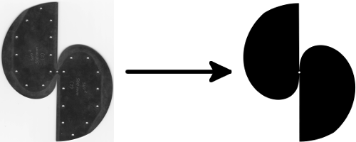
For the processing of the image several parameters should be defined:
-
Coordinates (in pixels) of the center of the sector. They can be estimated from the image manually.
-
Range of distances (in mm) from the center of sector, which should be processed.
-
Step size (in mm) for the processed distances.
Additionally, particular resolution values can be defined for the image, if they differ from the ideal values. Note, internally UNEX determines numerically the total sector function, which has values in the range [0,1]. This function is converted to the reduced sector function on the basis of the current sector model. Therefore it is advised to define explicitly a sector model, which fits your sector most closely. Remember, the determined reduced sector function is valid only for the model, which was defined in the processing of the sector image.
Below is an example of UNEX input for processing of sector image.
BASE=READ,<BASE>,</BASE>
IMAGE=SECTOR,Image0005.tif
PRINT=SECTOR
STOP

<BASE>
 imgfiles=Image0005.tif
 SecModelType=sinpn
 SecPrmN=2.0
 SecPrmRmax=75.0
 SecPrmA=1.412283
</BASE>

<Image0005.tif>
Xc=2950
Yc=3707
XResolution=1200.0
YResolution=1200.0
IntRfr=2.5
IntRto=75.0
IntStep=0.05
</Image0005.tif>
Data reduction
UNEX implements procedures for data reduction, i.e. for transformation of 2D images of measured diffraction patterns
to profile curves of experimental electron scattering intensity functions.
Images must be in uncompressed 8- or 16-bit grayscale TIFF format with little-endian byte order.
For introduction of images in UNEX the imgfiles keyword in BASE must be used.
The major procedure for data reduction [21] is started by command
IMAGE=INTSCAN,imgfile
where imgfile is the name of image TIFF file to be processed.
Before processing it is highly recommended to clean images. The cleaning procedure is essentially the setting of absolute white grayscale level to pixels, which do not correspond to the diffraction pattern itself (shadows, etc) or represent areas, which should not be processed due to any other reason (defects, etc). The Figure below demonstrates on the left side an initial image of a diffraction pattern with shadows due to construction elements in the diffraction chamber and a resulted image after cleaning. Note, graphical software used for these purposes should not alter values of valid pixels or change the bit depth. Check this before using the software in real investigations!

The other important issue in data reduction is the usage of correct calibration for the sanning device.
If the scanner produces uncorrected images the calibration should be taken into account on the stage of data reduction.
This includes the spatial calibration, i.e. setting the true resolution values in the input file using
keywords XResolution and YResolution. Note, the deviations of true from nominal resolution values can be different
in different scanning modes. This must be carefully investigated for the particular scanning device and scanning modes.
The other part of calibration is the correction of output signal.
For optical scanners the calibration of optical density is essential.
In this case optical wedges are processed for obtaining calibration curve specific for the particular device
(and possibly for the particular mode of operation), which is introduced in the input file for the data reduction, see Optical density section.
In effect, this kind of calibration must be done for any other type of scanning devices, for example for imaging plate scanners.
However, in this case instead of optical density the signal is calculated from pixel values using special formulae and
for calibration purposes appropriate standards are required.
IMAGE=INTSCAN procedure implements an iterative method [21] for refinement of parameters of diffraction patterns.
The maximal number of iterations can by adjusted with the keyword IntScanIter. For the processed image the following parameters should be defined:
-
Nozzle-to-detector distance,
NozToPlate. -
Step size for profile intensity grid,
IntStep. -
Electron wavelength,
IntLambda. -
Minimal and maximal distances from the center of diffraction pattern,
IntRfrandIntRto. -
Initial values for the coordinates of the center of the diffraction pattern,
XcandYc. -
If required, initial values for coordinates of the sector center can be defined, see
XsandYs. Otherwise they are initialized as equal toXcandYc. -
Optionally the signal (optical density) of unexposed areas can be defined using
fogkeyword. -
Parameters for the model of background,
ImgNbglX,ImgNbglYandMaxBgl. -
With keywords
MinTandMaxTit is possible to define a range of valid pixel values.
Note, some of these parameters can have reasonable default values while other must be defined explicitly. In the refinement a model of the pattern is created, which depends on the following parameters:
-
Coordinates of the diffraction pattern center.
-
Coordinates of the center of rotating sector device.
-
Values of total intensity on different distances from the center of diffraction pattern. They constitute profile of the diffraction pattern.
-
Values of background, defined on a grid (see keywords
ImgNbglXandImgNbglY) of the image.
Whether parameters of one or other type will be refined depends on settings of keywords IntVarCentre, IntVarSecCentre and IntVarAsymBgl.
Intensity values are always refined. The program also detects invalid pixels and sorts them out automatically.
The result of this procedure can be checked by inspecting image with weights of pixels.
In the end of diffraction image processing IMAGE=INTSCAN can create several images in TIFF format with refined profile,
background and weights for original image points. The images are created, if the respective parameters were refined and the
keywords WriteAsymBglImg, WriteWeightsImg and WriteCurveImg are set to appropriate values.
The names for images are constructed automatically as <basename>_profile.tif, <basename>_bg.tif and <basename>_w.tif, where
<basename> is the basename of the original input file of the processed image.
Note, these image files are created in the current directory.
Other operations with images
Histograms
UNEX can print histograms of images in numerical form, which can be useful for detailed analysis of data. For this the following command should be used
IMAGE=HISTOGRAM,imgfile
If at least one of keywords MinT or MaxT were defined for the processed image, then a new image is created with the name
<basename>_lvl.tif, where <basename> is the basename of the original image file.
In the created image the levels are adjusted by zeroing pixel values outside the range from MinT to MaxT
whereas the values of other pixels are rescaled to the full range depending on the bit depth of the original image.
The figure below demonstrates the effect.
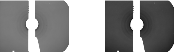
Comparing images
Comparison of images can be done with the command
IMAGE=COMPARE,img1,img2,...
where img1 and img2 are names of image files, which should be defined in BASE with keyword imgfiles as usually.
At least two images must be defined in the command. All images must be of the same size, bit depth, and photometric interpretation.
The procedure does a pixelwise averaging of pixel values and calculation of respective standard deviations.
In the processing two new images are created and saved in files <basename>_average.tif and <basename>_stdev.tif,
which correspond to the averaged image and the image representing standard deviations of pixels.
The <basename> is the name of the first processed file without extension.
Modification of ED intensity
The INT command can be used not only for introducing total experimental electron scattering intensity functions but also for their modification.
In this case the general syntax is
INT=jobtype,int1,[int2,int3,...]
where jobtype is the type of modification, int1 and possibly int2 and so on are intensity identificators.
The types of the modification are
-
S4MLT— multiplication by s4 function. -
INORM— calculates integral value of the total intensity and normalizes the intensity on this value. -
RSECDIV— divides the total intensity by the reduced sector function. -
SPLDIV— total intensity approximated by cubic spline and divided by this spline. By default number of inflection points for the spline is zero. This number can also be defined in the command. -
SMOOTH— smoothing total intensity using natural B-splines. -
SCALE— more than one curve must be defined, the first curve remains unchanged, the other curves scaled so that they fit the first curve best. -
TSCALE— intensity values are divided by t-factors from respective data sets. -
RESPCORR— correction using response function. The response function must be already refined or introduced with theRESPFUNCcommand, see Response function for details and example. -
COPYMODEL— copy data from the model I(s) intensity. This makes experimental I(s) equal to the calculated model I(s). -
ADDGNOISE— add Gaussian noise to existing experimental I(s). Standard deviations for the Gaussian distributions can be defined in input (see ED intensities) or calculated in averaging procedures.
Note, if standard deviations were defined for the total intensity, then their values are also modified accordingly.
For modifying experimental molecular intensity functions a similar command SMS with the same syntax exists
SMS=jobtype,int1,[int2,int3,...]
The available variants for jobtype are
-
SMOOTH— smoothing of molecular sM(s) intensity using natural B-splines. -
COPYMODEL— calculate and copy data from model sM(s) intensity. This makes experimental sM(s) equal to calculated model sM(s). -
ADDGNOISE— add Gaussian noise to existing experimental sM(s). Standard deviations for the Gaussian distributions can be defined in input (see ED intensities), calculated by various procedures (for example in averaging, combining and background procedures, see this manual) or estimated inMINIMIZE.
Models for ED intensity
In independent atom approximation total electron diffraction intensity can defined as [22]:

where Imol is its molecular part (i.e. function depending on molecular dynamics and geometry) and Iat is the atomic part — a function depending only on properties of atoms but not on their relative positions. In reality the measured total intensity also contains some additional extraneous additive background B:

Note, the total intensity and all its components are here per unit time, i.e. they are flux values. In real experiments signal is accumulated over finite time, so in general case the model for the total intensity must include a t-factor proportional to exposure time:

In this case Itot can be directly compared with experimental data. If rotating sector is used, it modifies the measured total intensity. Mathematically this can be defined using sector function S as

where M is the reduced molecular scattering intensity and β is the reduced additive background:

This model of Itot corresponds to the setting IModel=a1bgl.
For details on how sector function is defined and calculated see chapter ED sector function.
The other possibility is

which corresponds to the setting IModel=a2bgl.
In case of using multiplicative background (see chapter Multiplicative background) the model is set to IModel=mbgl
and the total intensity is calculated as

where k is the scale factor for the molecular intensity M and Φ is the multiplicative background.
Calculation of molecular intensity Imol depends on the setting of the keyword ImolAnhTermModel.
If ImolAnhTermModel=Morse then the formula is

where ij are the indices for the pair of atoms i and j, f is the scattering factor (see chapter ED scattering factors), l is the mean amplitude of interatomic vibrations, ra is the thermal-average interatomic distance, a is the parameter of the Morse anharmonic potential. The summation is performed for all pairs of atoms.
For ImolAnhTermModel=Asym the model is

The symbols here have the same meaning as above, except that the asymmetry constants κ are used. This is the default approximation. Note, the c3 constants from the cumulant approximation [17] (as printed, for example, by the ElDiff program [19]) are related to κ parameters as κ = c3/6.
Dynamic models
The formulae above for Imol are for semi-rigid molecules.
For non-rigid molecules dynamic models can be constructed using pseudoconformers
and defining potential energy function (see chapter Potential functions).
The molecular intensity is calculated according to DynImolModel setting for the respective molecule.
If DynImolModel=sum then Imol is defined as a weighted sum of molecular intensities of pseudoconformers:

here Pi and Imol,i are weighting factor and molecular intensity function for the pseudoconformer i.
The summation is performed over all N pseudoconformers.
The pseudoconformers are considered as semi-rigid and their respective Imol are calculated as described above.
UNEX explicitly implements one-dimensional dynamic models,
i.e. it is possible to choose one geometrical parameter as a coordinate φ for large-amplitude vibrations.
This is done assigning negative group number (usually -1) to the respective parameter in Z-matrix of the first pseudoconformer
(the assignment for others is done automatically).
All pseudoconformers have different fixed values of this dynamic coordinate and it is excluded from all refinements.
Its values are used for calculation of potential energies of respective pseudoconformers.
The weighting factors are calculated from potential energies using a variant of Boltzmann distribution:

where ki is the degeneracy factor of the pseudoconformer (see keyword sing),
Q is the normalization denominator (sum of all Pi calculated with Q=1),
V(φi) is the pontential energy of the pseudoconformer with dynamic coordinate φ=φi,
R and T are universal gas constant and temperature, respectively.
The other possibility is DynImolModel=integ. In this case the molecular intensity of a non-rigid molecule
is defined as the integral [23]:

In UNEX the integration is done numerically (using trapezoidal rule) from φmin to φmax
defined by respective pseudoconformers. Here P is the same Boltzmann distribution as above.
This last integ variant is computationally slightly more expensive but also more consistent in comparison to sum above.
It is recommended to use integ.
Mixtures
When the probe is a mixture of different species then the molecular and atomic scattering intensities are defined as weighted sums

where xi is the mole fraction of species i, Imol,i and Iat,i are molecular and atomic scattering functions of species i.
Values for mole fractions can be defined using keyword molx in information fields of respective molecules.
Note, they must be in range 0.0 — 1.0 and are constrained as

The complete reduced molecular intensity M(s) is defined in UNEX as

which is generally not equal to the less accurate approximation

Below is an extreme example of 1:1 mixture of CH4 and CI4 showing differences between two methods for calculation of complete M(s) function.

The figures demonstrate that the later equation significantly overweights the contribution of CH4 in the total sM(s). This can be even better seen on the corresponding radial distribution functions below.
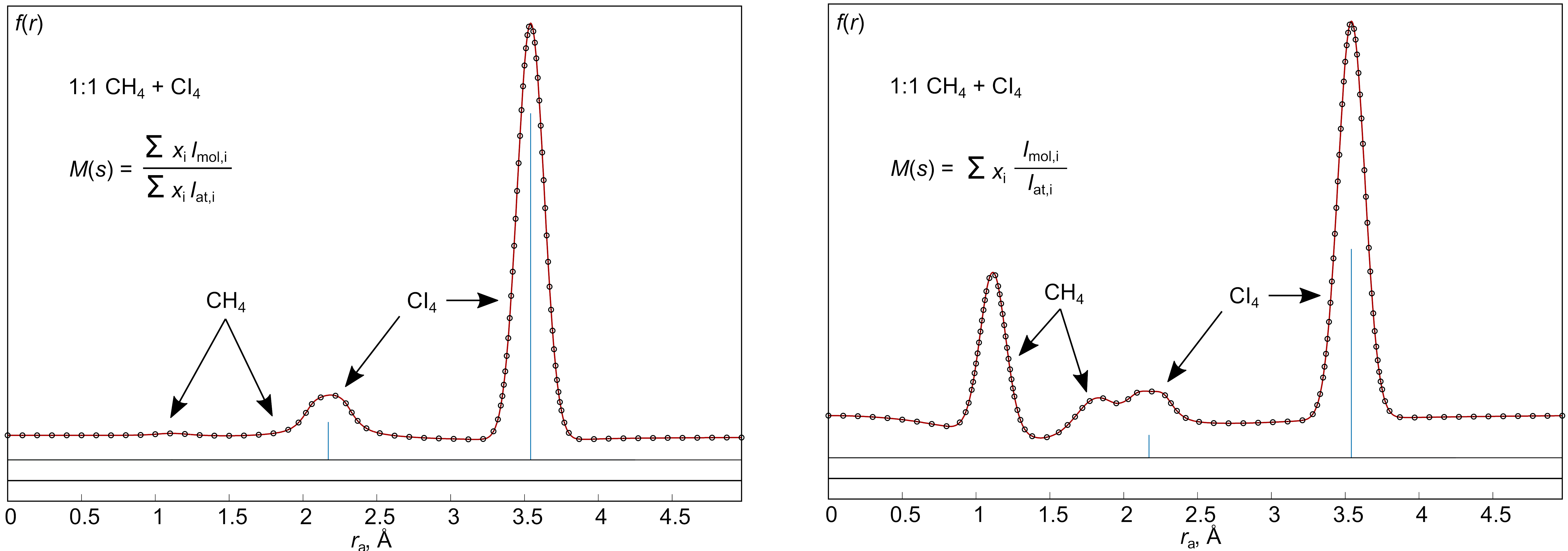
The figure on the left side correctly depicts the dominant contribution of CI4, whereas the signals from CH4 can hardly be seen. On the right is the RDF from molecular intensity calculated using the last inaccurate equation. Clearly the contribution of CH4 is significantly overestimated.
Note, both methods are equal for models of mixtures of species with equal empirical formulae. For example, this is the case for models of conformational mixtures.
ED background lines
Structural analysis in gas electron diffraction is performed on the basis of the molecular part of the total ED intensity. The molecular intensity is obtained by applying background elimination procedure. In UNEX are implemented models for two major types of backgrounds, multiplicative and additive. The later can be additionally defined in two variants.
Multiplicative background
Lets assume that the total intensity can be described by the model (see above)

This can be further modified to

From here an exact expression for the sM function can be easily obtained as

where function Φ is the so called multiplicative background, defined as

The advantage of the last expression for the sM is that it has no sector function S in explicit form. If the sector function is smooth (i.e. the sector device is of good quality) and experimental conditions result in smooth background β then the multiplicative background Φ must also be smooth. However, separation of the two smooth functions, β and Φ is a very ill-posed problem and in real practice an approximate formula is used for calculation of experimental sM function:

This expression becomes exact if extraneous background β is zero, which is never achieved in real experiments. However, in structural analysis, when model sM functions are fitted to the experimental data, scale factors for the sM curves are usually refined to compensate for this problem. If experimental sM curves are obtained by accounting for multiplicative background as shown above then the refined scale factors k can be defined as

Clearly, in real cases they are less than 1 due to positive β. The smaller is the background, the closer is k to 1. If refined scale factors are larger than 1, this is strong indication of deficiency of the theoretical model. It should also be mentioned that the presence of strong background does not necessarily lead to significant inaccuracies in the obtained experimental sM curve. Much worse is a possible deviation of the forms of the functions B and Iat, making β non-constant in the range of observable diffraction angles and, as such, not allowing for compensation with a single scale factor k.
Technically, multiplicative background is estimated on the basis of the calculated model molecular intensity sMmod. First, the model background is obtained from the equation

In real practice the calculated Φmod is not smooth and can contain oscillations due to inexact sMmod and experimental noise from the total intensity Itot. On the next step Φmod is smoothed using cubic splines [24] or fitted with a polynom by minimizing the functional

The obtained in this way smooth line is called experimental background Φexp and is used for calculation of the experimental molecular intensity

which can be afterwards used in structural analysis, for example in least-squares method. Thus, the background Φexp is in fact model-dependent and, as a consequence, the so called experimental molecular intensity sMexp is to some degree also model-dependent. To overcome this problem it is recommended to refine the model on the basis of the obtained sMexp and to use the updated sMmod for calculation of a new experimental background and a more accurate experimental sMexp. This procedure should be iteratively repeated until self-consistency.
In UNEX there is a command BGL for obtaining smoothed experimental
multiplicative background lines and corresponding experimental molecular intensities.
The general syntax of the command is as follows:
BGL=int1,int2,int3,...,intn [number] [keywords]
Here int1, int2 and so on are the identificators of the data sets, whose intensities need to be processed.
With the optional integer number can be defined the required amount of inflection points
for splines (see details in [25], this is default) or, alternatively, the
order of polynomial function used for smoothing of the background.
The less is the number, the smoother will be the calculated background line.
BGL command can also accept one or more keywords with respective values:
-
IModel— keyword for choosing the model of the background. Can accept optionsmbgl,a1bglanda2bgl. -
CalcSigma— boolen keyword (can accepttrueorfalse) for turning on or off the calculation of standard deviations of experimental sM(s). -
ApproxType— type of background approximation. Can be one ofSpline,PolynomandChebPolynom. -
CubSplQ— cubic spline Q-functional value, floating point number. -
Anchor— for defining anchor points. -
RBPSDThr— definition of threshold RBPSD for smoothing cubic spline.
Note, these keywords are optional and the particular settings for the BGL
procedure are determined at run time according to the priority scheme (from highest to lowest):
-
Keywords of the
BGLcommand. -
Settings of the data set, see ED intensities chapter.
-
Global settings.
For example, the most important setting, background model, can be defined in the BGL command using the IModel keyword.
If it is not indicated, the setting from the data set is checked. If it is also not defined,
then the setting of the global keyword IModel is used.
Note, not for all local keywords exist global or specific for data sets analogs.
CalcSigma can be used if there are reasonable standard deviations
(introduced on input or calculated at run time) for the experimental total intensity,
which should be propagated into standard deviations of the calculated in BGL
procedure experimental sM(s)
BGL=1-1,3 CalcSigma=true
ApproxType can be used for explicit choosing of the approximation type for the background.
However, in most cases the default Spline setting from the global keyword BglApproxType is the
most appropriate choice, unless something special is happening.
CubSplQ can be defined for spline approximation, if no other criteria for the background line
smoothness are required. With this keyword a particular functional value Q can be given,
for which a spline must be calculated.
No integer number should be given in the BGL command when CubSplQ keyword is used,
for example
BGL=1-1 CubSplQ=1.0e-5
Another criterion for the background smoothness is its relative power spectral density (RBPSD) in the range of structural frequencies.
This can be activated by using the RBPSDThr keyword, for example
BGL=1-1 RBPSDThr=-20.0
In this case a cubic spline will be used for approximation of the background and its smoothness will be adjusted iteratively
so that the final RBPSD will be not larger than the requested value (-20.0 in the example above).
UNEX also provides a possibility to control approximation of background lines with help of anchor points,
which can be defined in BGL commands using the Anchor keyword as triples of numbers. For example, the command
BGL=1-1,2 Anchor=1.0/0.5327/1.0;18.4/0.4851/1.0
starts the procedure for the calculation of background for the intensity curve 1-1.
Here with the Anchor keyword two triples of numbers are indicated. These are the anchor points.
The format of the Anchor keyword does not allow spaces or commas. The numbers may be separated by slashes \ and semicolons ;.
In each triple the first number is the argument s-value, the second is the background anchor value
and the third is its weighting factor.
Technically, the anchor points simply substitute corresponding points of Φmod,
so the anchor s-values must be also in the intensity data set.
The procedure should approximate background so that its calculated values are close to anchor points.
The larger are the weights of the anchor points, the closer the approximated background line will be to them.
Note, this is true for cubic spline and simple polynomial approximations, but not for Chebyshev polynomial approximation.
Also the final result may be influenced by possible constraint(s) on the amount of inflection points,
polynomial power, etc.
Finding optimal anchor points is in general a manual trial-and-error procedure.
The number of anchor points is not limited.
If several intensity curves are defined in one command they will be processed sequentially and independently. For example, the command
BGL=1-1,1-2,2
is equivalent to two sequential commands
BGL=1-1,2
BGL=1-2,2
As has been pointed out above the BGL command calculates model-dependent background
because of the usage of the model sM(s) function.
The recalculated background, and as a consequence, updated experimental sM(s)
can be used to refine model parameters, including scale factor(s) k for molecular intensity(-ies).
In UNEX it is possible to refine the best scale factors k internally in the BGL command.
This is an iterative procedure, which can be turned on by setting the keyword
BglRefScaleMaxIter to a some positive value, for example 30.
The convergence criterion of this procedure can be controlled by the optional keyword BglRefScaleTol.
The accuracy of refined molecular parameters directly depends on the accuracy of the used
experimental molecular intensity function [26].
In turn, the molecular intensity is the result of the background elimination procedure
and it is very important that the background is reasonably smooth.
Otherwise the frequencies in the experimental molecular intensity can be
significantly biased, which can naturally lead to biased refined parameters.
The quality of the background line depends on how the total intensity is levelled.
This property strongly depends on the form of the sector device used in the experiment.
Best of all if values of the total intensity are in a narrow range of values
for all observable diffraction angles.
In this case the default procedure for smoothing of background lines works well
and the amount of inflection points serves as a good indicator of the background quality.
However, this criterion is not significant if the intensity curve changes too quickly.
A possible solution of this problem is to smooth reduced
(divided by sector function and atomic scattering) background by setting BglSmoothReduced=1.
This requires introduction of a sector function.
Note, for this particular procedure the sector function must not be necessarily very accurate.
It is enough to define calculated values for your type of sector.
The most important is to ensure that this function is smooth and together with atomic scattering
lead to a well levelled reduced total intensity. The figures below demonstrate a case for the total intensity of CCl4.
The first two demonstrate results of the default procedure when only 3 inflection points are allowed.
It is hardly possible to assess the quality of the total background line (on the left side).
However, in the reduced form (on the right side) the relatively low quality of the background is getting clear.
In contrast, smoothing of the reduced background results in the line of much
superior quality as the figure below shows.
It should, however, be noted that higher quality background lines naturally lead to higher R-factors.

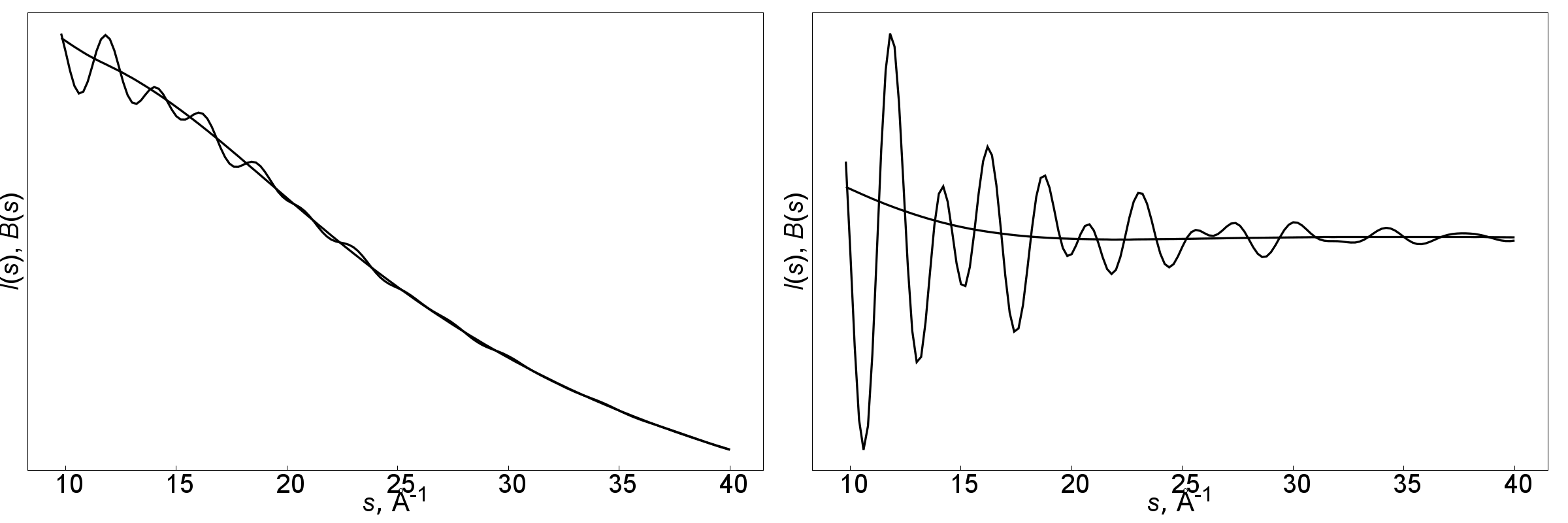
Additive background
Two types of additive background can be calculated in UNEX.
For the first type the model a1bgl of total intensity is used:

In can be calculated using the BGL command with the IModel keyword as,
for example
BGL=1-1 2 IModel=a1bgl
Note, the calculated background is

For the second type the model a2bgl is used, which is defined as

The corresponding UNEX command is, for example
BGL=1-1 2 IModel=a2bgl
In this procedure the background B is calculated.
Defining background type
Each invocation of any background command sets the respective type of model for the respective total intensity. For example, the commands
BGL=1-1,1 IModel=mbgl
BGL=1-2,2 IModel=a1bgl
BGL=1-3,3 IModel=a2bgl
internally set mbgl, a1bgl and a2bgl as models for the total intensities of the data sets 1-1, 1-2 and 1-3, respectively.
The same happens when background lines are introduced in numerical form using the command BGL=READ.
Thus the initial setting of the keyword IModel for the respective data set can be overriden.
A special form of the BGL command can be used for redefining the type of the model for total intensities:
BGL=SET,int
where int is the data set identificator.
For example, the commands
BGL=SET,1-1 IModel=mbgl
BGL=SET,2-1 IModel=a1bgl
BGL=SET,3-1 IModel=a2bgl
set the models mbgl, a1bgl and a2bgl for the total intensities in the sets 1-1, 2-1 and 3-1, respectively.
Averaging ED data
In UNEX there is a possibility for averaging ED intensity curves with an AVERAGE command.
The general syntax of the command is as follows:
AVERAGE=itype,int1,int2,...,intn [> oint]
Here itype is the type of intensity data to be averaged;
int1, int2 up to intn are identificators of intensity curves as input data for averaging;
> oint is the optional argument with explicit identificator for output averaged data.
Output data set oint must not necessarily by initialized before calling AVERAGE.
However, if it was already initialized, the data will be overwritten.
If you do not define oint explicitly then a new set of data will be initialized and its identificator will be printed to output.
itype can be one of the following:
-
INT— averaging total intensity curves -
INTS— averaging total intensity with calculation of standard deviations -
SMS— averaging experimental sM(s) intensity curves -
SMSS— same asSMSbut with calculation of standard deviations
Experimental sM(s) must be initialized, i.e. introduced in UNEX or determined in background procedure from total intensity.
If background procedure is used for curves with unrefined scale factors, it is advisable to set the BglRefScaleMaxIter keyword
in BASE to some positive value so that scale factors are adjusted to some reasonable values.
Note, averaged intensity values are calculated for s values of the first curve int1 defined in the command.
If points of the other curves are defined not in the same s values then interpolation with cubic splines is used.
In addition to averaging of data and optional calculation of standard deviations AVERAGE command also calculates
experimental R-factors [30].
For each of the curve, participating in averaging procedure, individual experimental R-factors are calculated as

where ![]() is the i-th point of the intensity curve, for which the R-factor is calculated,
is the i-th point of the intensity curve, for which the R-factor is calculated,
![]() is the corresponding point of the averaged intensity with weight wi,
N is the total number of intensity points.
Intensity I is the total intensity if
is the corresponding point of the averaged intensity with weight wi,
N is the total number of intensity points.
Intensity I is the total intensity if INT or INTS is defined, or sM(s) in case of SMS or SMSS.
Individual experimental R-factors show how much each of intensity curves deviates from the average curve.
This information allows to sort out curves of low quality. An average value of individual Rexp is also printed.
Regarding weighting, UNEX calculates two types of experimental R-factors:
-
with account of weights w, which are calculated from respective standard deviations of the averaged curve as
. -
without weighting, assuming all wi = 1.
Note, in INT and SMS modes standard deviations are not calculated so both types of experimental R-factors are equal.
Weighting works in SMSS and INTS modes, when standard deviations for the average curve are calculated.
Next UNEX calculates total experimental R-factor as

Here summation is performed for all points of all M intensity curves. I can also be total or molecular sM(s) intensity, depending on averaged data type.
The total experimental R-factor allows to represent numerically the overall reproducibility of experimental data and their general quality.
Weighted and non-weighted (setting all wi = 1) total and average experimental R-factors are calculated.
Note, the weighted experimental R-factors are calculated even if the standard deviations were not computed in this particular procedure.
They could have been defined or calculated earlier for the averaged data set.
Run PRINT=INTS or PRINT=SMSS for the averaged data set to see the values of standard deviations used for the calculation
of the weighted experimental R-factors.
The advantage of experimental R-factors based on total intensities is that no molecular model is needed for their calculation. However, the absolute values of such Rexp are generally meaningless. They can mostly be useful for comparison of data sets produced only by the same experimental setup. In contrast, experimental R-factors on the basis of sM(s) curves are directly comparable with structural R-factors:

where ![]() and
and ![]() are the experimental and model sM(s), respectively.
are the experimental and model sM(s), respectively.
Rstr indicates level of disagreement of the model with experimental data, while Rexp indicates reproducibility of experimental data. There can be several situations:
-
Rstr >> Rexp: data are reproducible but model cannot describe them; the model should be improved.
-
Rstr << Rexp: model describes data too well, probably not reproducible data features are fitted; better data are needed.
-
Rstr ≈ Rexp: optimal solution if both values are small.
Note, if both Rstr and Rexp are large, then something went completely wrong, first of all in experiment and/or in data reduction.
Also note that weighted Rstr (named wRd in UNEX output) should be compared with weighted Rexp, likewise non-weighted Rstr should be compared with non-weighted Rexp.
Below are several examples of averaging commands.
-
Simple averaging of intensity curves
1-1,1-2and1-3. A new average curve is created and assigned to an automatically chosen identificator.AVERAGE=INT,1-1,1-2,1-3
-
Same as above, but also standard deviations are calculated for the averaged data.
AVERAGE=INTS,1-1,1-2,1-3
-
Similar to the first example. Here the output average curve is accessible using the
1-4identificator.AVERAGE=INT,1-1,1-2,1-3 > 1-4
-
Averaging experimental sM(s) curves
2-1,2-2,2-3and2-4. The output data is written to3-1.AVERAGE=SMS,2-1,2-2,2-3,2-4 > 3-1
-
Averaging experimental sM(s) curves with calculation of standard deviations. The output data are written to a new automatically generated set with a new identificator. It is written in log file.
AVERAGE=SMSS,2-1,2-2,2-3,2-4
Combining ED data
Another possibility of converting multiple ED curves into a single curve provides COMBINE command.
It has exactly the same syntax as the AVERAGE
COMBINE=itype,int1,int2,...,intn [> oint]
but in general case does a different job creating a curve with s-values present in all input curves
(in contrast, AVERAGE takes points s only from the first input curve).
Thus, curves with different s-ranges can be combined together. For the overlapping areas averaged values are calculated.
If standard deviations were initialized for the respective input data sets, weighted averaging is used,
where weights are calculated as reverse squares of the respective standard deviations.
The Figure below demonstrates how COMBINE works for two experimental sM(s) curves obtained from different nozzle-to-detector distances.
The respective command was
COMBINE=SMS,1-1,2-1 > 3-1
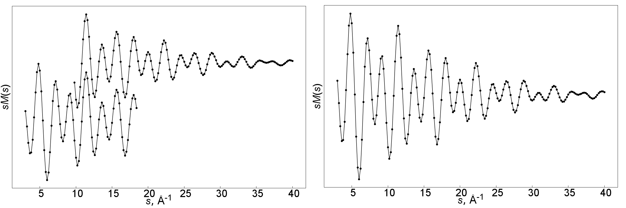
Note, in COMBINE experimental R-factors are calculated in a similar manner is in AVERAGE (see above).
There are, however, some peculiarities.
The weighted R-factors are also calculated if standard deviations were not requested for calculation.
However, in contrast to AVERAGE, standard deviations are still calculated internally, used for computation of wRexp,
but are not saved for the averaged data set. In this case calling PRINT=INTS or PRINT=SMSS is useless
for getting respective standard deviations. Also it should be noted that standard deviations are set to 1e99
if only one data set has contribution to the combined data in the respective point.
ED radial distribution functions
Radial distribution functions in UNEX are calculated and printed by the RDF command:
RDF=int1,int2,...,intn
The argument(s) of the command is a list of one or more ED intensity curves with initialized sM(s) functions. The calculation is essentially a sine-Fourier transformation of the respective experimental and model sM(s) curves:

If several curves are provided in the list of arguments, they are concatenated before Fourier transformation, for example
RDF=1-1,2-1
Note, the curves must have common range of s-values.
The concatenation procedure includes relative scaling of curves, re-interpolation to common argument values (if required) and weighted averaging in common ranges of argument.
Next, there are three general modes for calculation of radial distribution functions, which directly influence the minimal and maximal values of integration argument s.
The modes, controlled by the RdfType keyword in BASE, are as follows:
-
old, the most simple method, takes (combined) experimental sM(s) curve and performs integration in the range of s-values in which this curve is defined. The resulting radial distribution function usually looks not nice since integration starts from smin not equal to zero. -
classic, a more advanced method, in which experimental sM(s) curve is supplemented with respective model curve on the left side before integration. This is done in order to get an "experimental" curve, which starts from s=0. This, in turn, stabilizes integration and improves the overall appearance of the radial distribution function. Note, this makes sense if model sM(s) function fits well the experimental data. On the right side the experimental curve remains unchanged and integration is done till maximal s value for which the curve is defined. This can lead to problems with integration since at maximal experimentally achievable s-values of 30-40 Å-1 sM(s) functions are numerically not enough converged to zero. To overcome this problem the experimental sM(s) can be multiplied by an exponential function for damping, see keywordRdfDampin BASE. Note, this procedure leads to broadening of peaks on the radial distribution function and to reduction of its resolution. -
modern, the most advanced method, which supplements experimental sM(s) with model data not only on the left side as in theclassicvariant but also on the right side, so that smax is as large as possible (60 Å-1 in current implementation). This allows to avoid usage of damping exponential function and, as a result, leads to improved resolution of F(r). However, to obtain good results the model function must fit experimental data well.
Note, the concatenation of model and experimental sM(s) curves in classic and modern types of RDF requires some overlap of these functions.
The extent of the overlapping can be adjusted using keyword RdfNconcat.
Below are some examples of RDFs for benzene using different options of RdfType:
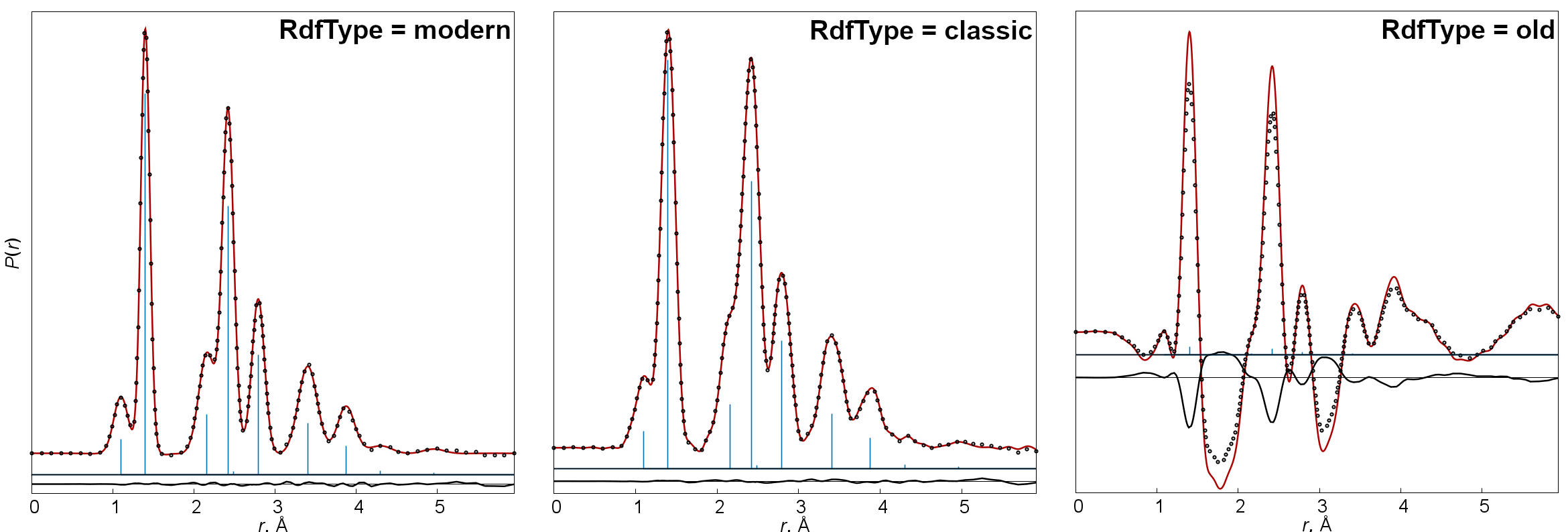
|
|
Below is the graphical representation of the influence of damping function on the RDF in case of benzene when RdfType=classic and experimental data available only up to 30 Å-1.
If the damping is turned off, i.e. RdfDamp=0.0, the RDF has multiple false peaks. An optimal value of damping factor removes these peaks.
Too large value of the damping factor increases widths of true peaks so that the resolution of RDF is too low.
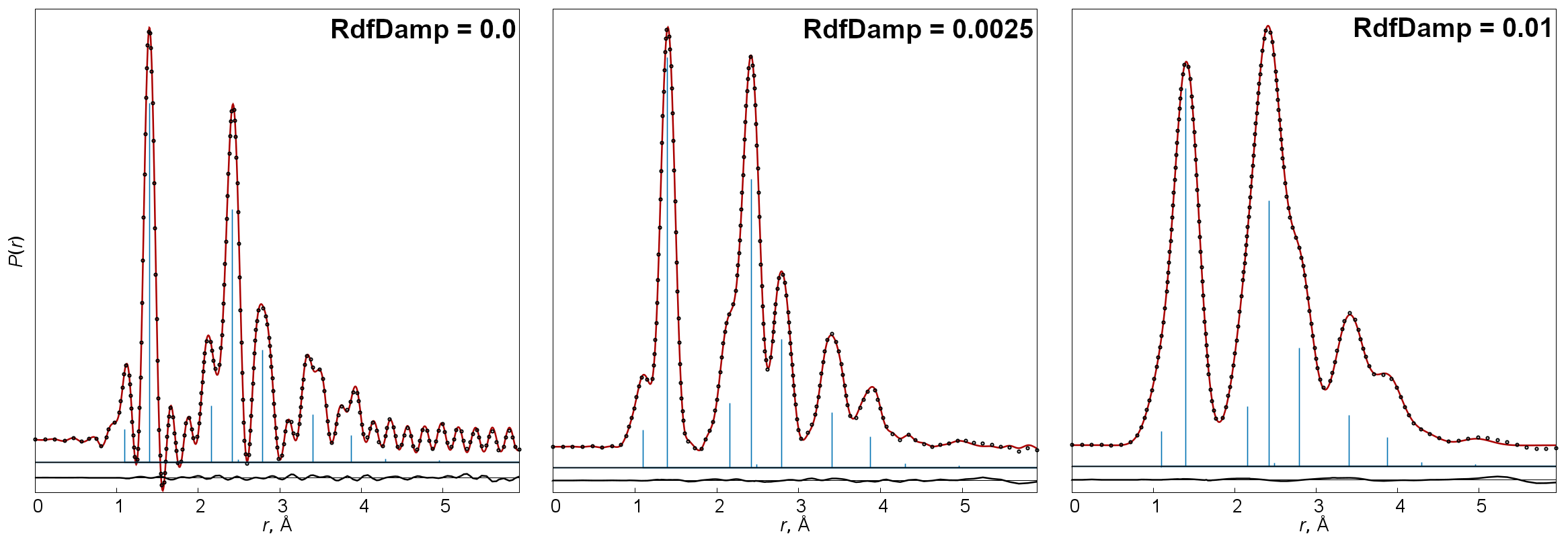
The next issue in calculation of RDF is connected with representation of contributions of different terms in sM(s) functions. In a crude approximation the contribution of a pair of atoms to diffraction pattern is proportional to the product of their atomic numbers. The respective RDF in this case can be easily analysed.
In reality, however, contributions of atomic pairs to diffraction patterns are not constant on the s-scale and are even not linear (this property is characterized by g-functions). As a consequence, the calculated RDF is difficult to analyze. Fortunately, ratios of many g-functions for different types of atoms are much closer to constants than g-functions themselves. Therefore UNEX provides a possibility to divide the integrated sM(s) data by a g-function, see RdfDivGf keyword in BASE. This can improve the appearance of the obtained RDFs. By default for this purpose UNEX chooses g-function for the pair of atoms with maximal product of atomic numbers. Note, however, that this logic can fail in molecules containing atoms with very different atomic numbers. In this case some g-functions can go through zero and change sign. Accordingly, RDF cannot be obtained by integration of sM(s) modified by such a g-function. In this case an optimal g-function can be chosen manually by using RdfDivGfAtoms keyword.
In case of benzene the influence of RdfDivGf is as follows:
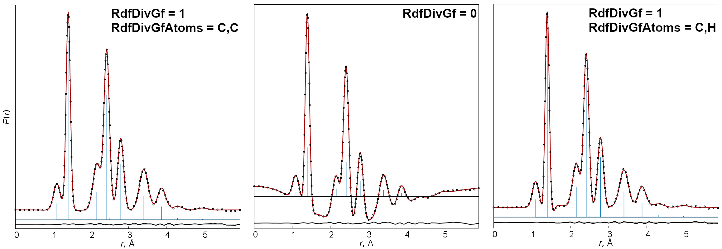
For obtaining RDFs integration is done numerically. For this UNEX implements two methods, simple trapezoidal and more accurate but slower Romberg method. In most cases the first method is accurate enough and is used by default. Switching between integration methods is done by RdfIntegMethod keyword in BASE.
Regarding r-values, for which RDFs are calculated, two schemes are implemented in UNEX:
-
If
RdfAdaptiveR=1(by default it is=0, i.e. turned off) the so-called adaptive step size is used depending on the local curvature of the RDF in each point so that obtained function is accurate enough for numerical analysis. -
For purposes of visual analysis RDF is calculated on a fixed grid on the r-scale, where step is determined by the
RdfRdrkeyword. However, for better appearance some points can be skipped, so that in general they are arranged nearly equally dense along the RDF line and not along the r-scale. This is default and controlled by theRdfPruneRlenkeyword. To turn off the prunning of points setRdfPruneRlen=0.0.
The RDF defined above as integral F(r) is essentially the distribution P(r)/r, where r is the distance between atoms and P(r) is its distribution function. The first moment of the function Pij(r)/r for a particular pair of atoms ij is the ra type of thermally averaged distance between these atoms. Thus, RDFs calculated as described above show peaks centered at ra distances. There is, however, a possibility to obtain RDF defined as P(r), which is more natural. For this, UNEX can multiply the integral by r, see RdfMultR keyword. In this case the peaks are centered at rg distances between atoms. Note also that this procedure naturally increases the difference curve (difference between model and experimental RDFs) proportionally, so this should not be misinterpreted as a worsening in the model fit.
Below is such an example using data for Ph-CH2-CH2-CH2-Se-CF3 molecule. Note again, both RDFs were obtained for exactly the same experimental data and model.
The advantages of the P(r) function are clearer physical meaning and more distinct visibility of contributions from terms with large interatomic distances.
In contrast, the P(r)/r function effectively hides discrepancies between data and model, which hinders analysis.
Therefore in UNEX the default setting is RdfMultR=1 so that P(r) RDFs are generated.
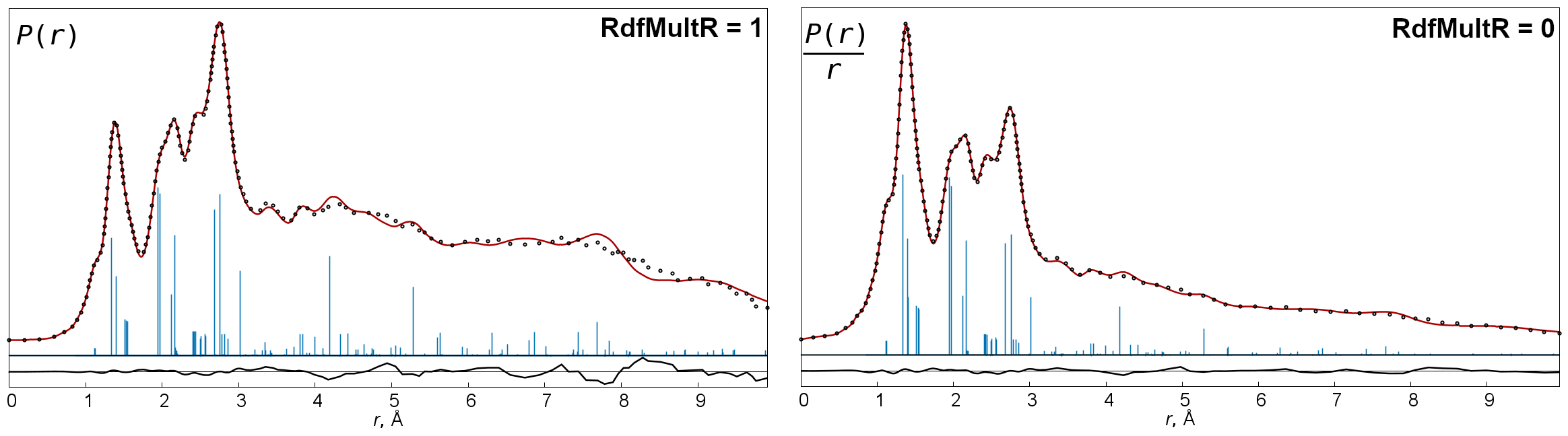
|
UNEX can also calculate pure model radial distribution functions if the |
If your experimental molecular intensities have meaningful standard deviations it is possible
to calculate errors of experimental RDFs by switching the RdfCalcStdevs keyword on.
Standard deviations for sM(s) can be defined in input file as absolute values,
calculated in averaging procedure or in background procedure from respective errors of total intensity functions.
Standard deviations for sM(s) are also estimated in MINIMIZE but should be used with care in case of large R-factors.
Note that the calculated values of standard deviations for RDF’s only represent random errors
propagated from respective errors of sM(s).
The default method for calculation of standard deviations uses error propagation formula and numerical
differentiation of sM(s) functions. For large models the calculations can be (very) time consuming.
There is an alternative procedure which uses the Monte-Carlo method. This can be activated by setting the keyword
RdfMCEsdIter to some positive integer value, indicating the number of iterations.
It is recommended to investigate the convergence of the calculated results with respect to the number of iterations.
In some cases the optimal value of RdfMCEsdIter can be from several hundreds to several thousands.
Below in Figure simulated molecular intensity functions for 1,2-dichloroethane (1:1 mixture of anti and gauche conformers) are shown. Random Gaussian noise, with standard deviations 0.03 for the curve above and 0.025 for the other curve, was added to the simulated experimental data.
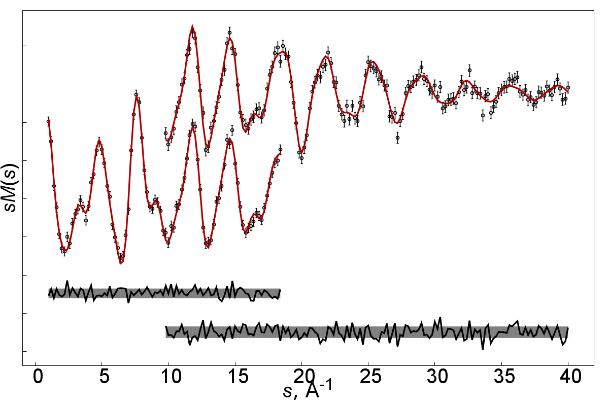
These data were used to calculate model and experimental RDFs with respective standard deviations. The obtained data are plotted on the Figure below. Note, the calculation was done with RdfMultR=1, that is RDFs corresponding to P(r) were calculated. Therefore oscillations of the difference curve and the standard deviations increase when r increases.
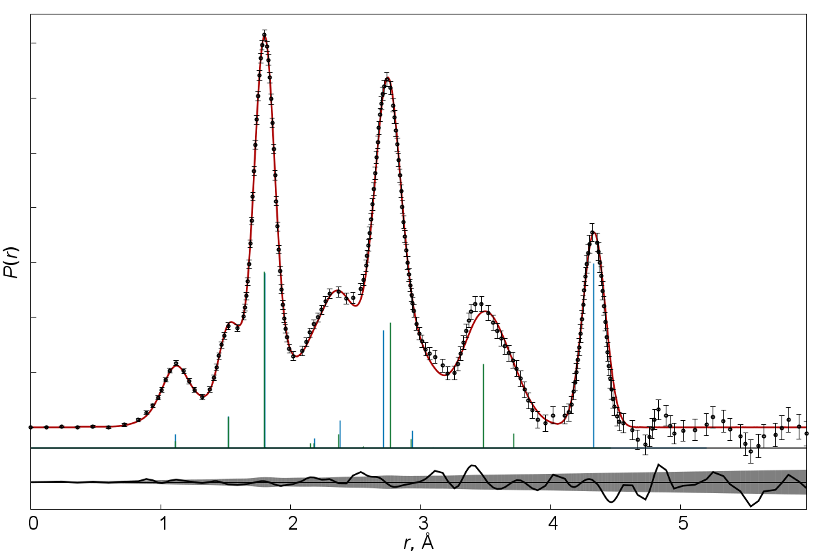
Alternatively UNEX can calculate more traditional RDFs of type P(r)/r by switching the RdfMultR keyword off. Usually in this case standard deviations are distributed approximately equally along r scale. The Figure below demonstrates P(r)/r for 1,2-dichloroethane calculated from the simulated sM(s) data shown above.
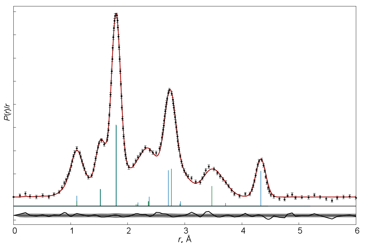
|
For graphical interpretation of RDFs it is useful to print also interatomic terms and their contributions with |
Models for rotational constants
In the simplest case, model rotational constants are computed by diagonalizing inertia tensors,
which are calculated for the current geometrical structure and using atomic masses located in infinitesimal points.
The type of the structure is determined by user, for example it may be equilibrium.
This model is called "rigid rotor - point atomic masses" and corresponds to the setting RotConstModel=rrpatm:

The other option, RotConstModel=rrpatm-vibc, in addition utilizes input vibrational corrections,
defined by the keywords RotA_vibc_value, RotB_vibc_value and RotC_vibc_value.
First, the "rrpatm" values are calculated, from which the respective vibrational corrections are subtracted.
Note, the correction is defined as

typically

Thus, the model rotational constant is calculated as

The third option, RotConstModel=rrpatm-elc1-vibc, adds an electronic correction in addition to the vibrational correction.
The electronic correction is calculated as (for details see the book of W. Gordy and R. L. Cook [31] page 548)

where ![]() is the axis in the principal system,
is the axis in the principal system,
![]() is the effective model rotational constant,
is the effective model rotational constant,
![]() and
and ![]() are the rotational constants
calculated using atomic (the "rrpatm" definition) and nuclear masses, respectively,
m and M are masses of the electron and proton, respectively and
are the rotational constants
calculated using atomic (the "rrpatm" definition) and nuclear masses, respectively,
m and M are masses of the electron and proton, respectively and
![]() is the corresponding diagonal element of the rotational g tensor.
Thus, using UNEX designations (and omitting the axis symbols for simplicity) the total model rotational constant is calculated as
is the corresponding diagonal element of the rotational g tensor.
Thus, using UNEX designations (and omitting the axis symbols for simplicity) the total model rotational constant is calculated as

The diagonal components of the rotational g tensor are defined using the keywords RotG_gaa_value, RotG_gbb_value and RotG_gcc_value.
Note, in the actual calculation automatically corrected g values (gcorrected) can be used,
if respective relative shifts were also defined, RotG_gaa_rshift, RotG_gbb_rshift and RotG_gcc_rshift.
The definition for these shifts is

Accordingly, the corrected g value is calculated as

Refinement of molecular parameters
Refinement of all kinds of parameters in UNEX is closely associated with the term group.
Group is a list of parameters tied by particular constraints.
Most often the constraints are fixed differences between values of parameters within each group.
In case of vibrational amplitudes for interatomic distances there is also a possibility to fix their ratios within each group instead of differences (see GedVarAmplScale keyword).
The number of parameters in a group is not limited. However, only particular kinds of parameters can be grouped together.
Formally a group can also consist of only one parameter.
In this case the respective parameter is not tied to any other parameter in refinement procedures.
Groups are defined by unique integer numbers. Each parameter can be defined with its respective group number.
Several parameters with the same group number are combined together to a single group and
refined with fixed constraints.
By default parameters are defined without group numbers, which is the same as to define the group number to 0.
If you want to refine parameters, you have to define their group numbers larger than zero explicitly.
For refinement procedures the amount of variables is equal to the number of active groups.
Thus, multiple parameters in a group in fact act as a single parameter in least-squares refinement.
Consequently they share the same estimated standard deviation as a group,
not as they had individual but equal standard deviations!
Below is the list of parameter types, which can be refined in UNEX.
-
Geometrical parameters of Z-matrices. See respective chapter on how to assign group numbers to these parameters. Parameters of the same type can be combined together in a single group, for example a distance can be combined only with other distances. It is generally impossible to combine different types of geometrical parameters into a group. However, it is allowed to combine angles and torsional angles. Note, geometrical parameters of different molecules can be tied together in one group.
-
Interatomic distances ra can be refined independently. See
GEDTERMScommand on how to define respective groups. -
Vibrational amplitudes of interatomic pairs. Respective groups can be defined in the same fields as the values for amplitudes. Alternatively, there are possibilities to group amplitudes (semi-) automatically after their definition (see below). Amplitudes in different molecules can be grouped together.
-
Mole fractions for molecules in mixtures, see parameters
molxandvarxin molecular fields. -
Parameters of potential functions in dynamic GED models of molecules.
-
Scale factors for GED molecular intensity functions, see the
VarSckeyword in field of intensity curves.
Semi-automatic grouping of amplitudes can be done using AMPLGROUP command.
AMPLGROUP=mol,gstart, r1s,r1e, r2s,r2e, ...
Here the grouping is done for the molecule mol. The numbering of groups starts from the number gstart.
The parameters r1s and r1e should be floating point numbers, defining range of distances in the molecules.
Amplitudes of terms, whose ra distances are within this range, are grouped together.
Multiple ranges can be defined, r2s and r2e above indicate the second range.
In the following example
AMPLGROUP=mol,200 1.4,1.6 2.0,3.0
amplitudes of terms in mol with ra distances between 1.4 and 1.6 Å are assigned to a group with the number 200.
Next, amplitudes of terms with ra distances in the range from 2.0 to 3.0 Å are assigned to a group with the number 201.
Another possibility is the fully automatic grouping of amplitudes for all molecules
in the model with AUTOGROUP command:
AUTOGROUP=AMPLITUDES
This procedure calculates internally a radial distribution function (RDF) for the current ED model
and assigns equal group numbers for amplitudes of the terms, which reside within single particular peak of the RDF.
Accordingly, this method requires completely initialized ED model.
In real practice it is strongly advised to analyse the performed by this procedure grouping and adjust it manually if need.
Also note, both AUTOGROUP and AMPLGROUP procedures perform grouping only for those amplitudes
which had previously group numbers equal to zero.
MINIMIZE
UNEX provides several refinement procedures. The most important one is the least-squares (LS) method.
The minimization of LS functionals can be done with the MINIMIZE command, with the common syntax
MINIMIZE=functional(s) [data] [groups]
The type of functional is the required parameter of the command, data should be defined in case of ED, groups can be defined or prohibited explicitly but this is optional (see below). There are several types of functionals:
-
GEDSMS— molecular part of electron diffraction intensity in form of sM(s). -
ROTCONST— rotational constants. -
REGPRM— regularization parameters, also known as flexible constraints or restraints. -
RESTRGEOM— restraining geometrical parameters.
In most general form the complete functional is represented as

Here the first, second, third and fourth terms correspond to GEDSMS, ROTCONST, REGPRM and RESTRGEOM types of functional, respectively.
The relative global weight factors αrot, αreg and αrgp are defined by the keywords RotConstAlpha, RegAlpha and RestrGeomAlpha, respectively.
If GEDSMS is given, particular ED intensity curves must be indicated explicitly for constructing functional, for example
MINIMIZE=GEDSMS,1-1,2-1
Individual weights wi for the sM(s) data points are calculated automatically from their standard deviations
as wi=σi-2.
The other types of functional do not require explicit indication of their data. ROTCONST automatically includes all defined
rotational constants for all molecules and for their isotopologues, see keywords RotA_exp_value, RotB_exp_value and RotC_exp_value.
The weights are calculated in the same manner as for ED data from respective standard deviations defined with keywords
RotA_exp_stdev, RotB_exp_stdev and RotC_exp_stdev.
Functional REGPRM uses data, which can be read in using the respective
command REGPRM. The syntax of the command is:
REGPRM=mode,otag,ctag
The only available mode of the command is INPUNEX, which means reading of the data as in the following example:
REGPRM=INPUNEX,<myregparams>,</myregparams>

<myregparams>
1     1.490     0.001
2   110.0       0.1
3     0.05      0.01
</myregparams>
Here in the first column group numbers are indicated. In the second and third columns regularization values and their individual standard deviations are defined. In the equation above the regularization values correspond to pkreg, while the weights wk are calculated from the introduced standard deviations as wk=σk-2.
|
In UNEX versions before 1.6-1273 the values in the third column are interpreted as weights, not as standard deviations! |
Note, the regularization is applied to first parameters in groups, so the regularization values must be appropriate.
The other parameters in the groups are regularized automatically to the same extent due to rigid constraints.
Regularization must not necessarily be used for all refined parameters, restraints can be applied to some selected groups.
With REGPRM it is possible to define regularization parameters for groups, whose parameters are not refined.
In this case the respective restraints are ignored and not included in least squares functional.
This is because in different MINIMIZE (or in SEARCH and others) procedures different groups of parameters can be refined,
whereas the list of regularization parameters is global.
The units of the regularization values must be the same as the units used for introduction of respective model parameters.
For parameters of potential functions internal UNEX units must be used. They can be checked by printing data using PRINT=POTENTIAL.
RESTRGEOM functionals are built on the basis of geometrical parameters of molecules.
The allowed types of parameters are interatomic distances, angles, torsion angles and out-of-plane angles.
For definition of parameters and numeration of atoms see section for geometrical parameters in chapter Data printing.
The restraining data are read in for particular molecules with RESTRGEOM command as in the example:
RESTRGEOM=mol,INPUNEX,<rgeom>,</rgeom>

<rgeom>
bond       1    2                0.970   0.010
bond       2    3                1.385   0.005
bond       3    4                1.200   0.002
bond       3    5                1.185   0.002
angle      1    2    3         103.1     0.5
angle      2    3    4         115.6     0.5
angle      2    3    5         114.1     0.5
angle      4    3    5         130.1     0.5
torsion    1    2    3    4      0.0     0.00001
o-o-p      5    3    2    4      0.0     0.00001
</rgeom>
In each line first a string with type of parameter is given. The possible types are bond
(dist and distance can also be used as synonyms), angle, torsion and o-o-p (for out-of-plane angles).
Next, numbers of atoms must be defined. Finally, values and respective standard deviations for the defined parameters are given.
Note, the standard deviations are optional but it is recommended to indicate them explicitly. Otherwise they are assumed to be 1.0.
The units for distances and angles are Angstroms and degrees, respectively. In LS functional the weights are calculated from the defined here
standard deviations σ as wl=σl-2. Note, for models of mixtures each molecule can have
an individual set of restraining geometrical parameters. All of them are participating in the same respective sum in the LS
functional given above. The prefactor αrgp is thus the same for all sets.
In should be noted that restraining geometrical parameters should not necessarily be equal to the parameters in
definition of molecular geometry, which can be refined in MINIMIZE (or in other procedure).
Also, distances can be given for chemically non-bonded atoms.
In the beginning of the MINIMIZE procedure the information on data for constructing the LS functional is printed.
This include number of data, α values, etc. If electron diffraction intensities are used, then
the structural resolution and maximal structural distance are estimated. The former is calculated as

where smax and smin are the maximal and minimal s-values for which experimental ED intensity values are available. The maximal structural distance is calculated as Nyquist frequency due to the Whittaker–Nyquist–Kotelnikov–Shannon sampling theorem [41, 42]:

where Δs is the average spacing between adjacent intensity data points in Å-1. The rmax value shows the largest interatomic distance, which can possibly be determined from the current electron diffraction data set.
Minimization of the LS functional can be done using two methods:
A particular method to use (or a combination of methods) can be chosen with the MinMethod keyword.
All methods are iterative, the maximal allowed number of iterations is defined by keyword MaxIter.
Iterations stop in several cases:
-
Relative change in functional is less than threshold value (see keyword
LsqFunTol). -
Maximal relative parameter addition is less than threshold value (see keyword
LsqAddTol). -
Maximal relative gradient (partial derivative of functional with respect to some refined parameter) is less than threshold value (see keyword
LsqGrdTol). -
Parameter
Lambdain Levenberg-Marquardt method increased too many iterations in a row (see keywordLsqLamMaxInc). -
Maximal allowed number of iterations performed.
In UNEX there are two different weighting schemes in LS analysis: relative and absolute.
They influence calculation of standard deviations of refined parameters.
With absolute weights the matrix of covariances (with squares of standard deviations of parameters as diagonal elements)
is obtained directly as inverse of normal matrix.
In case of relative weighting the calculated cofactor matrix (the inverse of the normal matrix) is multiplied by the factor
χ2/v, where v is the number of degress of freedom, calculated as the number of data points minus the number of
refined parameters v = Ndata - Nprm.
The switching between absolute and relative weighting can be done using the MinAbsWeighting keyword.
Depending on settings MINIMIZE can print different types of data for information on minimization status, properties,
convergence and so on:
-
Total absolute and relative values of functional χ2 designated in output as
X^2. The relative values are printed during iterations of solving LS problem. In this case the initial value of the functional is scaled to be 1.0 and the following values are relative to this initial unity. -
Lambdais the parameter in Levenberg-Marquardt method [43, 44] for improving convergence. Stable minimization is accompanied with decreasing of this parameter. -
RfandwRdare printed in case of using electron diffraction data. The first one is the regular R-factor calculated without weights:
The other,
wRd, is the R-factor with diagonal weighting:
Note, on iterations total wRd values are printed, i.e. the summations are performed for all data points of all intensity curves, if several are used. Individual different types of R-factors for particular intensity curves are printed after minimization.
-
RMSDandWRMSDare root-mean-square and weighted root-mean-square deviations, respectively. For rotational constants they are calculated as
where N is the total number of rotational constants, and

Analogous formulae are used for other types of data. During iterations WRMSD for rotational constants and all restraining geometrical parameters are printed in columns
RotWRMSDandRgpWRMSD, respectively. -
When regularization data are used, the respective part of the total functional (see equation for χ2 above) is printed as
RegQ.
After minimization several blocks of data are printed:
-
Information on the convergence of the procedure.
-
Statistics for the data and model:
-
Number of degrees of freedom (number of data points minus number of refined parameter groups).
-
Condition number (ratio of maximal and minimal singular values of normal matrix). Large values can indicate numerical instability.
-
Rank and nullity of the design matrix in LSQ method.
-
Goodness-of-fit value printed in case of absolute weighting. It is defined as 1-Q, where Q is the probability that the functional χ2 should exceed its refined minimal value by chance. Small values (close to zero) of goodness-of-fit can indicate that (i) model is not adequate, (ii) standard deviations for data points are probably larger than stated, (iii) measurement errors are not normally distributed. On the other hand values of goodness-of-fit close to or equal 1 can indicate that defined standard deviations of data points are too large/pessimistic.
-
Values of functional parts.
-
For sM(s) data different R-factors (diagonal-weighted
wRdand without weightsRf), RMSD/WRMSD, estimated standard deviations for the data (seeESDin output), etc. -
For electron diffraction sM(s) data the Durbin-Watson statistics [46, 47] are printed (indicated as
DW). -
Also, unweighted R-factors (for each curve separately and total) are calculated and printed for M(s). However, they are provided mostly for the completeness and for a possible comparison with results from other programs. Normally, for the assessment of the data fit, it is recommended to use the R-factors calculated for sM(s) data.
-
-
Table with refined parameter values, their absolute and relative errors and partial derivatives of total functional with respect to these parameters. Errors of parameters are least-squares standard deviations multiplied by factor
PrintEsdFactor. -
Optional tables with contributions of functionals to refined parameters (see
CalcFuncProportionkeyword). Note, here errors (standard deviations possibly multiplied by a factor) and respective so-called experimental errors of the refined parameters are also printed. The experimental errors are defined and calculated as described in [6]. KeywordMinSigmaExcludeFunccan be used to control this method. -
Matrix of correlations.
-
Table with correlations above 0.5, if there are any.
-
Optional table with χ2 (hyper)ellipsoid (see
MinPrintEllipsoidkeyword).
Several types of functional can be combined in MINIMIZE. For example, the following command
MINIMIZE=GEDSMS+ROTCONST,1-1,2-1
refines parameters from rotational constants and indicated ED data simultaneously. In the same manner three types of data can be used
MINIMIZE=GEDSMS+ROTCONST+REGPRM,1-1,2-1
or with restraining geometrical parameters
MINIMIZE=GEDSMS+ROTCONST+RESTRGEOM,1-1,2-1
Other combinations are possible.
As already stated refinement of particular parameter groups can be (dis)allowed. By default all parameters with group numbers greater than zero are refined. If group numbers are defined explicitly in MINIMIZE then only parameters in these groups will be refined. The following example demonstrates how to refine parameters only in groups 1 and 2.
MINIMIZE=GEDSMS,1-1 1,2
The other possibility is to prohibit refinement of parameters from particular groups. In the following example parameters from all groups except group 5 are refined:
MINIMIZE=GEDSMS,1-1 !5
Several groups can also be excluded from refinement:
MINIMIZE=GEDSMS,1-1 !5,!6,!26
Combinations of permisive and prohibitive definitions of groups are meaningless. The command
MINIMIZE=GEDSMS,1-1 1,!2
is equivalent to
MINIMIZE=GEDSMS,1-1 1
i.e. refines parameters only from the first group.
OPTALPHA
In case of relative weighting of data in least-squares functional the factors
αrot, αreg and αrgp should have appropriate values.
The problem is that there is no single clearly defined criterion for optimal values of these factors.
Usually they are adjusted according to specific requirements of a particular investigation
(see discussion of the problem in [48]).
There are, however, some heuristic criteria. One of them is implemented in UNEX
[49] (a more detailed description is given in [6]).
The respective command is OPTALPHA:
OPTALPHA=functional(s) [data] [groups]
The syntax above is the same as for MINIMIZE. In fact this is an iterative procedure,
which internally starts MINIMIZE on each iteration.
Note, the procedure is implemented only for some cases when two types of functional combined together.
|
Always analyse result(s) of this command. Check whether the obtained alpha parameter fits your needs. In many cases it can be used only as a starting point for further search of optimal values. |
|
This procedure does not refine any parameters except respective α. That is, any other types of parameters,
including molecular geometry, remain unchanged after this command. Also, standard deviations and correlations are not determined.
Thus, if you run only |
ROBUSTM
The described above command for minimization of LS functionals implements the main procedure in UNEX for these purposes.
A more complex method is provided by the ROBUSTM command. In contrast to MINIMIZE it modifies weights of
experimental data using bisquare weights scheme of Tukey [50, 51]. Accordingly, standard deviations of data points are adjusted.
The weights are calculated iteratively from respective residuals. In fact ROBUSTM internally starts MINIMIZE procedure on each iteration,
refines model and updates weights of all data points. This procedure is repeated until weights are converged or the limit for number of
iterations is achieved (see MinRobMaxIter keyword). As the last step a normal minimization is performed and results are printed as
usually from MINIMIZE. The syntax for ROBUSTM is the same as for MINIMIZE:
ROBUSTM=functional(s) [data] [groups]
|
By design |
SEARCH
MINIMIZE and ROBUSTM are local methods for optimization of models.
This means that they typically converge to local minima depending on starting approximation.
With these methods there is no possibility to know exactly whether obtained solution corresponds to global minimum on the functional (hyper)surface.
For this purpose in UNEX there is a special command SEARCH, which provides two methods.
The first one implements a systematic scanning of functional by testing different values of parameters in defined ranges.
The syntax of the command is as follows:
SEARCH=SCAN,functional(s),otag,ctag,[data]
Here functional and data are defined exactly in the same manner as for MINIMIZE command.
The opening and closing tags otag and ctag are for data field with information on which parameters should be used in scanning procedure.
The format of the data field can be best shown by example:
<scan>
2   1.76   100    1.78
4   0.04   100    0.06
</scan>
This is definition of a two-dimensional scan. Each line defines a parameter or a group of parameters, which should be scanned.
Here the first line is for group number 2. The first parameter in this group should be scanned in range from 1.76 to 1.78
(other parameters in this group will be automatically adjusted using fixed constraints) with 100 steps.
In the same manner scanning for the second group (in the example group number 4) is defined.
In total, the two-dimensional scan will do 100x100=10000 calculations of functional for different combinations of parameters.
After this UNEX reports statistics for parameters:
-
Values of paramaters (first parameters in respective groups) which correspond to minimal value of total functional.
-
Weighted statistics for each parameter:
-
Mean value.
-
Standard deviation.
-
Skewness.
-
Kurtosis (but not excess kurtosis).
-
-
Minimal tested value.
-
Maximal tested value.
In addition UNEX prints weighted correlations between parameters.
|
Accuracy of weighted statistics (including correlations) can be sensitive to the size of scanned area and to the number of tested points. In particular, area in the vicinity of minimum of functional must be sampled dense enough in oder to get well converged values of statistics. Otherwise values of skewness and kurtosis are printed as zeros if they cannot be calculated accurately. The sign for this is a very small value of respective standard deviation. In case of numerical problems with calculation of correlations respective rows and columns and diagonal elements are printed as zeros. Otherwise diagonal elements are exactly 1. In many cases to get reasonable values of statistics at least several tens of thousands points are required. To test for convergence you need to recalculate the values for at least twice as large number of scanned points. |
The procedure in SEARCH=SCAN finds global minimum of functional within defined limits for values of parameters and with accuracy determined by scanning step size(s).
The problem is, however, that the required number of scanning points scales as SN, where S is the number of steps for each parameter and N is the number of parameters or groups of parameters.
Thus, the total number of points increases very quickly with the number of scanning dimensions.
To avoid this problem UNEX implements Monte-Carlo method for searching of global minimum of functional.
The syntax of the respective command is very similar to that shown above. The only difference is that RAND should be indicated:
SEARCH=RAND,functional(s),otag,ctag,[data]
The definition of search parameters is also the same as in the example above.
For compatibility purposes the integer values (number of steps in case of SCAN) between minimal and maximal allowed parameter values
are also indicated but do not play any role and simply ignored by UNEX.
In case of RAND the amount of sampled points is controlled by time allowed for SEARCH, see SearchTime keyword.
Uncertainties of parameters
In inverse problems parameters are refined with uncertainties. After each least-squares refinement standard deviations and correlation factors are calculated for parameters. They can be accurate in a simplest case, when the only source of uncertainty is the noize in experimental data and under condition that an appropriate weighting for experimental data is used. However, in real practice uncertainties in other parts of the refined model can propagate into uncertainties of the refined parameters.
A possible way to take this into account is to use the direct Monte-Carlo simulation approach [52]. This method is implemented in UNEX and can be started by calling the command MCMIN:
MCMIN=functional(s) [data] [groups]
This command has the same syntax as MINIMIZE described above.
In fact, the MCMIN procedure calls MINIMIZE internally as a first step. After its convergence the Monte-Carlo procedure is started. Parameters and/or data are sampled randomly from respective distributions and for the newly generated model and data a least-squares method is started for minimization of defined in MCMIN command functional. The refined values of parameters are saved. These steps are performed multiple times in a loop. Thus statistics for refined parameters are collected and the procedure is repeated until convergence or until the maximal allowed number of iterations is reached.
The following data can be randomized:
-
Experimental data (if
MCRandData=1is defined inBASE).-
Experimental molecular scattering intensity functions. For details see below.
-
Experimental rotational constants, see keywords
RotA_exp_pdf_p1,RotA_exp_pdf_p2(and analogous for rotational constants B and C) in molecular field. -
Regularization parameters, which indeed can be experimental from some other source or they can be assumed values with some defined absolute standard deviation.
-
-
Model parameters (if
MCRandParams=1is defined inBASE).-
Parameters defining background spline smoothness, see keywords
MCBglQ,MCBglQMinandMCBglQMaxin field for scattering intensity. -
Electron wavelengths, see keywords
MCLamandMCLamSin input field for scattering intensity. -
Geometrical constraints (fixed values of parameters and their differences), see below command
ZMATMC. -
Fixed amplitudes of interatomic vibrations or their differences and ratios, see command
TERMSMC. -
Vibrational corrections for interatomic distances, see command
TERMSMC. -
Relative abundances of molecules in mixtures, see keywords
MCvarx,MCxMinandMCxMax.
-
There are several possibilities on how electron diffraction intensities are randomized.
-
In case of absolute weighting (
MinAbsWeighting) each point is sampled from a gaussian distribution with respective standard deviation and centered on original experimental value of this point. -
If standard deviation is defined for sM(s) globally with the keyword
MCsMsSpreadthen this value is used for all points. -
Otherwise are used estimated standard deviations for each curve independently from the initial least-squares run. Note, within each curve all points have the same value of standard deviation.
The first variant is the best if accurate standard deviations are known for molecular intensities.
For rotational constants the only option is to define directly standard deviations in molecular field(s) using keyword RotA_exp_pdf_p2 (analogously for constants B and C).
The random values are sampled from respective Gaussian distributions centered on original experimental values.
The initial state of used internally random number generator can be controlled using the keyword MCRandDataSeed.
Set this parameter to a particular integer value if you want to obtain reproducible results.
Otherwise it is initialized automatically in a pseudo-random manner so that you get numerically different results in each run.
However, if the procedure is well converged the results must be very similar.
For randomization of parameters group numbers are used.
If a parameter should be randomized an integer group number should be assigned to this parameter using special keywords (MCBglQ, MCLam, MCvarx) and/or commands (ZMATMC, TERMSMC).
Parameters in the same groups (with equal group numbers) are randomized so that differences between their values are kept fixed.
This is similar to refinement of parameters, when only those parameters are refined, which have non-zero group numbers.
The rules for combination of parameters in groups are the same as for refinements.
|
The group numbering systems for refinement and for randomization are completely separated, so you can use the same numbers for these two purposes. However, it makes no sense to randomize parameters which are subject to refinement. |
For grouping of Z-matrix parameters ZMATMC command is used:
ZMATMC=mol,type,otag,ctag
where type defines type of limits for minimal and maximal parameter values, which is one of ABS, ABSDEV or PERC.
The input field for this command should consist of four columns: name of parameter from Z-matrix of the current molecule, randomization group number for this parameter and two floating-point numbers defining limits for randomization. If type is ABS then absolute minimal and maximal values should be defined, like in the example:
<ZM_mol_MC>
   F1       1    150.0  180.0
   F2       2      0.0   60.0
</ZM_mol_MC>
Here F1 and F2 are names of torsion angles, which have been defined earlier in a Z-matrix for a molecule. These two angles will be randomized independently in two separate groups with group numbers 1 and 2. The first angle will be randomized in the range from 150.0 to 180.0 degrees, the other angle will be randomized in the range [0,60]. Note, parameters are sampled from uniform distributions with defined minimal and maximal values.
If type is ABSDEV then deviations from current values of parameters are defined in the input field, for example:
<ZM_mol_MC>
   F1       1     10.0   15.0
   F2       2      5.0   10.0
</ZM_mol_MC>
After reading of this data the limits for randomization of F1 are [VF1-10,VF1+15], where VF1 is the current value of F1. The limits for randomization of F2 are [VF2-5,VF2+10].
If type is PERC then deviations are defined in percents from current values of parameters, for example:
<ZM_mol_MC>
   F1       1      0.5   0.5
   F2       2      1.0   1.0
</ZM_mol_MC>
Here the limits for F1 are in fact [VF1-0.5*VF1/100,VF1+0.5*VF1/100], where VF1 is the current value of F1. Similarly for F2 the limits will be [VF2-1.0*VF2/100,VF2+1.0*VF2/100].
Note, command ZMATMC does not require that all Z-matrix parameters are listed in the respective input field. It is enough to indicate only those parameters, which should be randomized.
|
Note, for correct calculation of biases the refined parameters must be already optimal for the given functional before starting the |
Information required for randomization of ED vibrational amplitudes and corrections is introduced with the TERMSMC command:
TERMSMC=mol,type,otag,ctag
Here type can be one of AMPLPERC, CORRPERC, AMPLABS, CORRABS, AMPLABSDEV and CORRABSDEV. Prefixes AMPL and CORR indicate amplitudes and corrections.
Suffixes ABS, PERC and ABSDEV indicate that the data are introduced as absolute values, as percent deviations from current active values or
as absolute deviations from current values. This scheme works in the same way as in the ZMATMC command.
Below is an example for CO2 molecule:
TERMSMC=mol,AMPLPERC,<MC_ampl>,</MC_ampl>
TERMSMC=mol,CORRPERC,<MC_corr>,</MC_corr>

# In percent!
<MC_ampl>
C2   O1    201  35.0   35.0
C2   O3    201  35.0   35.0
O1   O3    202  35.0   35.0
</MC_ampl>

# In percent!
<MC_corr>
C2   O1    301  500.0   500.0
C2   O3    301  500.0   500.0
O1   O3    302  500.0   500.0
</MC_corr>
UNEX provides a (semi)automatic procedure for collecting statistics on minimal and maximal values of parameters (Z-matrix parameters, vibrational amplitudes and corrections), which can be printed in a way suitable for later introducing in Monte-Carlo procedure. This is demonstrated in the example below:
RESTERMSTATS # Reset statistics for ED terms
# Collect stats
MOLXYZ=mol,XYZUNEX,<XYZ1>,</XYZ1>
AMPLITUDES=mol,FREEU,<AMPL1>,</AMPL1>
UPDPRMSTATS # Update stats after each reading of new parameter values
MOLXYZ=mol,XYZUNEX,<XYZ2>,</XYZ2>
AMPLITUDES=mol,FREEU,<AMPL2>,</AMPL2>
UPDPRMSTATS
# Print stats as templates with infos for MC
PRINT=ZMATMCTMPL,mol
PRINT=AMPLMCTMPL,mol
PRINT=CORRMCTMPL,mol
The idea consists in reading different sets of geometrical parameters (here in form of Cartesian coordinates, which update Z-matrix parameters)
and vibrational amplitudes and corrections.
The first command RESTERMSTATS is used for resetting of statistics.
Next new parameters are introduced in a usual way.
After reading of data the command UPDPRMSTATS is used for updating of parameter statistics taking into account the freshly introduced values.
This can be repeated multiple times. In the end the collected minimal and maximal values are printed by PRINT=ZMATMCTMPL,mol, =AMPLMCTMPL and =CORRMCTMPL.
Note, by default the printed ranges of parameters are extended by particular factors, see documentation for these printing commands.
With slight modifications these data can be used as input for MC procedure.
|
The data and grouping of parameters in the printed in this way templates should be carefully analysed before using in Monte-Carlo procedure. |
During the MC procedure in intermediate and in final calculations of parameter statistics two methods can be used depending on the setting of the MCWeightedStats keyword,
i.e. the statistics can be calculated with and without weighting factors.
In the former case the weights are calculated as

where χ2i is the absolute minimized value of the least-squares functional on the i-th iteration of the Monte-Carlo procedure.
ED standards
UNEX can process ED intensities of gas standards. In most cases this is done in order to refine electron wavelength.
The respective command is STANDARD:
STANDARD=method,int1,...
Here method can be SCANLAM, REFINELAM or LSQ. Also in the command there must be defined one or more identificators of intensities,
which should be processed. For each intensity the type of standard can be defined with the keyword Std,
otherwise default value from the global keyword StdDefType will be used.
In most cases initial value of the electron wavelength (keyword Lam) and distance from nozzle to detector (keyword NtoP) must be defined.
It is also recommended to set sector to detector distance (keyword StoP) to an appropriate value
if sector device was used for obtaining experimental data and sector function is used in the procedure.
The first method SCANLAM does searching of the best electron wavelength by scanning.
The control keywords for this method are StdScanIter, StdScanLamMin and StdScanLamMax.
The other method REFINELAM searches the best electron wavelength using golden section method.
In contrast to the simple scanning it recalculates background on each iteration, which increases the overall accuracy of the obtained electron wavelength.
The most important keywords for this method are StdRefLamMaxIter and StdRefLamTol.
Note, the type of model for total intensities in these both methods can be chosen using individual for each intensity curve
keyword IModel. In fact this determines the type of background calculated for the intensities.
The valid options are mbgl, a1bgl, a2bgl and none.
The last option none explicitly indicates that no background should be calculated.
The background and respective experimental sM(s) are also not calculated if IModel is not defined.
In this case the experimental sM(s) must be defined and available from some other source, for example from input file.
The approximation for background lines can be defined using global keyword BglApproxType.
The flexibility of the lines can be controlled by defining the maximal number of inflection points with
the keyword BglNinflThr for each curve individually, or with the global keyword BglNinflThr.
If polynoms are used for background approximations, then the relevant local and global keyword is BglPolPow.
Depending on the type of background scale- or t-factors can be refined if StdBglRefScaleMaxIter is greater than zero.
The other option for the method is LSQ [53].
In this case the least-squares method is used.
It refines parameters of total intensities by minimizing a functional, which is generally defined as

The summation in the first term is performed for all points of all intensity curves processed simultaneously.
The second term is for regularization of the refined sector function,
if the keyword StdRegSecAlpha is set to non-zero value and a regularizing sector function is defined with the REGSEC command.
The third term is for regularization of refined background functions.
For this the StdRegBglAlpha keyword must be set to some non-zero value.
The regularizing value itself is defined by the keyword StdRegBglValue.
The fourth term is for the additional control of the background flexibility,
if the keyword StdRegDBglAlpha is set to non-zero value.
In fact this is a sum of second derivatives of backgound values of all curves in all points.
Again, the used model for the total intensity depends on the setting of the IModel keyword for each intensity curve.
In the least squares method the valid options are a1bgl and a2bgl. For details see Models for ED intensity.
In the first model background β is refined, in the second case background B is refined.
The reduced sector function is modelled numerically as a set of its values at particular r-values at the sector plane.
The particular set of r-values with explicit initial approximation for the reduced sector function can be defined with the SECTOR command.
Alternatively UNEX can automatically initialize initial reduced sector function, see keyword StdInitSecStep.
Note, in any case a model sector function must be defined, see SecModelType and SecPrm* keywords.
Backgrounds β or B are modelled as Chebyshev polynomials.
The order of polynomials can be defined for each curve individually using the StdModBglPow keyword.
Normally an initial approximation for the background is obtained by fitting the polynomial to a background,
which is obtained by running internally the BGL procedure.
This can be turned off by setting StdInitRefBgl=0.
The types of parameters to be refined is determined by the StdVar* set of keywords.
|
Refinement of background, sector function and other parameters in |
Diffraction intensities of the following molecules can be processed in UNEX as gas standards (default standard values are taken from the cited papers):
Currently used standard values of parameters for these molecules can be printed with the command
PRINT=STDPARAMS
It is also possible to define a custom set of standard parameters for each standard molecule with the STDPARAMS command:
STDPARAMS=stdtype,STDTERMS,otag,ctag
Here stdtype is the type of standard, one of the following: CCl4, C6H6, CO2, CS2.
In input file between tags otag and ctag must be defined types of terms and their parameters:
ra distance, amplitude l and asymmetry (or Morse) constant.
Note, the last parameter should correspond to your setting of the ImolAnhTermModel keyword.
By default it is ImolAnhTermModel=Asym, so asymmetry parameters are expected.
Model molecular intensity functions are calculated from these parameters using the respective approximation as described in chapter Models for ED intensity.
In these calculations multiplicity factors (number of equal terms of a given type in a molecule) are used automatically.
They are predefined for each term in each type of standard molecules in UNEX.
Here are examples of STDPARAMS command:
STDPARAMS=CCl4,STDTERMS,<ccl4terms>,</ccl4terms>
<ccl4terms>
    C-Cl   1.7667  0.0496  5.0e-7
  Cl..Cl   2.8892  0.0712  6.0e-7
</ccl4terms>
STDPARAMS=C6H6,STDTERMS,<c6h6terms>,</c6h6terms>
<c6h6terms>
    C-C    1.397760  0.046360  5.5e-7
   C..C    2.418800  0.055180  8.1e-7
   C..C    2.792300  0.058980  0.0
    C-H    1.095600  0.077060  0.0
   C..H    2.158700  0.099850  0.0
   C..H    3.404100  0.096880  0.0
   C..H    3.879200  0.093380  7.0e-8
   H..H    2.483300  0.157990  0.0
   H..H    4.300200  0.133170  0.0
   H..H    4.964400  0.118180  0.0
</c6h6terms>
STDPARAMS=CO2,STDTERMS,<co2terms>,</co2terms>
<co2terms>
    C-O    1.16419  0.0327  3.0e-7
   O..O    2.32427  0.0393  2.9e-7
</co2terms>
STDPARAMS=CS2,STDTERMS,<cs2terms>,</cs2terms>
<cs2terms>
    C-S    1.559    0.040   7.7e-7
    S-S    3.112    0.052   8.8e-7
</cs2terms>
|
The input order of the terms is important and must be as in the examples above. |
|
The values in the examples are only for demonstration of the input syntax. Do not use them in real investigations! |
Vibrational analysis
In UNEX it is possible to do a simple vibrational analysis.
Direct vibrational problem — calulation of harmonic vibrational modes and frequencies can be solved using the command VMOD as
VMOD=mol,DIAGF2MC
This runs a procedure, which diagonalizes the matrix of harmonic force constants in mass-weighted Cartesian coordinates.
Note, the force constants, as well as the respectively oriented Cartesian coordinates of atoms (and their masses!) must be already available in UNEX.
For this, for example, the commands F2C and MOLXYZ can be used.
Results of the procedure can be printed using the PRINT=VMODMC command (see below).
Force constants
In UNEX there are methods for converting cubic force constants between Cartesian and normal coordinates, as described in Ref. [56]. The respective commands are
F3C=mol,CONVF3N
and
F3N=mol,CONVF3C
The first command does a calculation of cubic force field in Cartesian coordinates from cubic force constants in normal coordinates. The last command does the opposite conversion.
Thermodynamics
UNEX can calculate thermodynamic functions using statistical thermodynamics theory [57].
For this the THERMO command should be used:
THERMO=STAT,mol [Optional parameters]
Geometry and vibrational frequencies should be defined for the respective molecule before running this command.
The frequencies can be calculated or introduced with the VMOD command (see Vibrational modes).
Depending on the ThermoModel setting of the molecule the calculation can be performed in different ways.
In the simplest case, ThermoModel=sRRHO, UNEX uses the model of ideal gas, assumption on uncoupled translational,
rotational and vibrational motions, rigid rotator and harmonic oscillator (RRHO) approximation [58].
Note, the frequencies may be scaled by using the ThermoFreqScale keyword, which turns the approximation effectively into the anharmonic oscillator, respectively.
The other option, ThermoModel=msRRHO-1, utilizes the so called modified scaled RRHO method by S. Grimme [12],
with a modified procedure for the calculation of the vibrational entropy. Two keywords are related to this method, ThermoMSRRHOWcutoff1 and ThermoMSRRHOWalpha1.
Note, this method was also known as quasi-RRHO [11].
The last option, ThermoModel=msRRHO-2, in addition to the entropy correction (as in msRRHO-1) uses also similar correction to enthalpy as described in [13].
The respective control keywords are ThermoMSRRHOWcutoff2 and ThermoMSRRHOWalpha2.
Thermodynamic functions are calculated for conditions (temperature and pressure) defined by optional parameters to the command (see below) or by global parameters.
In calculations it is also assumed that only the ground electronic state is populated and other states are not achievable.
The contribution of the ground electronic state is determined by the spin multiplicity and
can be defined using the SpinMult keyword in the field of the respective molecule.
The possible optional parameters of the THERMO command are as follows
- Temperature
- Pressure
-
Temperature (in K) and pressure (in atm), for which the thermodynamic functions must be calculated. By default they are initialized to the values of the global keywords
TemperatureandPressure. - CalcTrans
- CalcRot
- CalcVib
- CalcEl
-
Parameters for turning on and off the calculation of particular contributions to thermodynamic functions due to translational, rotational, vibrational and electronic motions, respectively. Each parameter accepts either
true(default setting indicating to do the corresponding calculation) orfalse(turn off).
For example, the command
THERMO=STAT,h2o Temperature=500.0 CalcTrans=false
calculates thermodynamic functions for the h2o molecule at 500 K and default (standard) pressure. All types of motions will be taken into account, except for translations.
On the output are printed inner energy U, enthalpy [H(T)-H(0)], entropy S, Gibbs free energy G,
constant volume heat capacity Cv and constant pressure heat capacity Cp.
The particular contributions to the thermodynamic functions and to the molecular partition function Q
from different types of motions are also printed.
If the electronic energy has been defined for the molecule (see the ElEnergy keyword) then total values for the thermal energy,
enthalpy and Gibbs free energy are printed.
Note, small vibrational frequencies lead to large errors in calculated thermodynamic functions within standard RRHO approximation.
Depending on the application, it may be reasonable to ignore such frequencies by using the keyword ThermoFreqCutoff.
However, a more universal way for solving this problem is to use the msRRHO methods.
Molecular trajectories
Technically the term molecular trajectory is here defined as a set of geometries for a molecule.
For UNEX it must be represented as a file in the standard XYZ format, in which sets of Cartesian coordinates follow one after another.
A single set of Cartesian coordinates within trajectory is called frame.
Trajectories can be obtained, for example, from molecular dynamics and Monte Carlo simulations.
For their processing UNEX provides different functions, invoked by the TRJXYZ command.
Distributions of geometrical parameters
A set functions is used for analysing distributions of geometrical parameters:
TRJXYZ=DIST,N1,N2,file.trj
TRJXYZ=ANGLE,N1,N2,N3,file.trj
TRJXYZ=TORSION,N1,N2,N3,N4,file.trj
TRJXYZ=OOP,N1,N2,N3,N4,file.trj
In these functions particular distances, angles, torsions and out-of-plane angles can be analysed. N1, N2, N3 and N4 are atom numbers, which define the required geometrical parameter.
file.trj is the name of the input file with the trajectory. For example,
TRJXYZ=ANGLE,1,2,3,ccl4.trj
will calculate the angle on atoms 1-2-3 for each frame in the trajectory in file ccl4.trj.
An analysis of the collected set of angles will be performed.
Finally on the output the statistics of the respective distribution are printed: mean value, standard deviation, skewness and kurtosis.
Additionally, sample size and the flag indicating weighted statistics are printed after SSize= and TrjWeightedStats=.
The weighted statistics are calculated if this is defined with the TrjWeightedStats keyword in the BASE input field
and the trajectory file contains special factors as X2=number in title lines for each frame.
Such trajectories are produced by UNEX when running Monte-Carlo simulations and X2 represents the value of least-squares functional χ2.
Depending on the keywords TrjScaleTotalQ and TrjShiftTotalQ the weighting factor for geometrical parameters of the particular frame is calculated as

Statistics may be calculated for all internal geometrical parameters simultaneously by running
TRJXYZ=ALLGEOM,file.trj
In this case a table is printed with parameters for all determined geometrical parameters of the molecule.
During trajectory processing distribution for a particular geometrical parameter can be printed to file.
This can be done by using the Dataout keyword in the particular TRJXYZ command, as in the example
TRJXYZ=DIST,1,2,ccl4.trj Dataout=dist12.dat
Here the file dist12.dat is created with a list of values for the distance 1-2 from each frame in the trajectory ccl4.trj.
Calculation of ED terms
Trajectories from molecular dynamics (MD) simulations can be used for calculation of ED terms [59, 60, 61]. More precisely this concerns vibrationally averaged interatomic distances ra and rg, mean amplitudes of vibrations l and asymmetry constants κ. The vibrationally averaged interatomic distances are normally used for calculation of respective vibrational coorections (re - ra) required in structural analysis. Processing of MD trajectories for these purposes in UNEX can be done by the following command:
TRJXYZ=EDTERMS,file.trj [Parameters]
The available parameters are
- Mols
-
The mandatory parameter indicating the list of molecules (separated by
;symbol), already defined in UNEX for which ED terms are to be calculated. The molecules must be of the same formula and related to each other as isomers or conformers. In the simplest case a single molecule may also be indicated here. - Dumpfile
-
Basename for file(s), in which terms of molecule(s) are printed for each trajectory frame.
- NwinTstFr
-
Trajectory window size (number of frames) in convergence testing. The default value is 1000.
- AmplThrEps
- CorrThrEps
- KappaThrEps
-
Convergence thresholds for amplitudes, distance corrections and asymmetry constants. These parameters define normalized (i.e. relative) root-mean-square deviations in the testing window (see
NwinTstFrabove). By default they are equal to 0.01, which corresponds to 1 %. - Symmetrize
-
A flag (
trueorfalse, default) indicating whether ED terms must be symmetrized. The symmetrization is done within all terms of all processed molecules. Symmetry elements must be already determined for each molecule, for example by runningPRINT=SYMMETRY,mol. Symmetry equivalent terms within each molecule are determined exactly. Equivalent terms in different molecules are determined approximately, see the parameterSymMaxDrbelow. - SymMaxDr
-
Maximal allowed difference between symmetrically-equivalent interatomic distances in different molecules. Note, comparison of distances is done only for pairs, which have the same types of atoms. Default value is 0.00001.
- CmpOldTerms
-
This is for comparison with old values. A flag (
trueorfalse, default) for enabling printing of newly calculated ED terms together with previously defined values.
The calculation of ED terms requires that for molecules have already been defined Cartesian coordinates,
for exmple by using the MOLXYZ command.
Normally they correspond to the equilibrium structure at the same level of theory, which has been used in obtaining MD trajectory.
Data printing
Normally UNEX by default prints status of executed commands and some summarized results of these commands.
There is, however, a special command PRINT for outputting different kinds of data.
This command can be executed at any stage of data processing.
The only requirement is that the respective data must be already initialized at the time of requesting printing.
In many cases UNEX prints values of parameters with respective errors from least-squares refinement or other procedures. Some parameters are not directly refined but rather calculated from values of other parameters. Such parameters are called dependent. Standard deviations for dependent parameters are calculated using the formula for error propagation

where f is the dependent parameter represented here as a function of independent parameters pi with standard deviations si
and covariations ρij, N is the number of groups of parameters.
By default UNEX uses covariations if they are available from latest least-squares refinement. This can be turned off with DepSigmaCovar keyword.
Standard deviations for independent parameters si are normally those from latest least-squares refinement or Monte-Carlo simulation.
However, in some cases they can be defined directly in input file. For example, values of parameters of Z-matrices can be introduced together with respective standard deviations.
Below is the description of different variants of the PRINT command.
General information
For getting current settings use
PRINT=INFO
Brief information about hardware and operating system is printed by
PRINT=COMPINFO
For information about loaded images you can use
PRINT=IMGINFO
Molecular symmetry
The command below prints symmetry elements for mol and respective point group. Geometry for mol must be already defined.
PRINT=SYMMETRY,mol
Rotational constants
PRINT=ROTCONST,mol
The command prints experimental and model rotational constants for mol.
Model values are calculated for the current geometrically consistent structure of mol.
Experimental values are printed as defined in the input.
Additionally, for each rotational constant respective corrections (defined earlier in the field of the molecule),
experimental standard deviations, differences between experimental and corrected (using input corrections) model values
and errors are printed. The errors are calculated on the basis of standard deviations of refined molecular parameters
using error propagation formula. In the end the values of root-mean-square deviation (RMSD) and weighted RMSD
(WRMSD, taking into account experimental standard deviations) are calculated and printed.
Note, (W)RMSD are printed only if at least one experimental value is not zero.
Vibrational data
Force constants can be printed by
PRINT=F2CMATRIX,mol
PRINT=F2CSHRINK,mol
PRINT=F2CGAMESS,mol
These variants print harmonic force constants in Cartesian coordinates for mol. The difference is in the format of printing.
Below is the command for printing cubic force constants in Cartesian coordinates.
The number of columns in each block is controlled by the F3cBlockCols keyword.
PRINT=F3CBLOCKS,mol
Cubic force constants in normal coordinates can be printed using the command
PRINT=F3NIDXLIST,mol
By default the constants are printed in internal units Hartree amu-3/2 Bohr-3.
However, it is possible to get the values in cm-1 by using the appropriate Units keyword:
PRINT=F3NIDXLIST,mol Units=cm
Vibrational modes in mass-weighted Cartesian coordinates and respective frequencies can be printed as
PRINT=VMODMC,mol
Each command also prints the particular units of the output data.
UNEX can prepare input data for DISP and ElDiff, the programs for vibrational spectroscopy and electron diffraction written by Igor Kochikov [19].
PRINT=DISPINPXYZ,mol
PRINT=DISPINPINT,mol
The first example prints data used as input for calculations in ElDiff using Cartesian coordinate system. The second command prints data for calculations in internal coordinates. Note, to be able to print such data there must be introduced harmonic and optionally cubic force field(s) and Cartesian coordinates for the respective molecule.
Geometrical parameters
Particular geometrical parameters of molecules are printed by calling PRINT command with options DISTANCE
(aliases are DIST and BOND), ANGLE (short variant is ANG), TORSION (short variant TORS) and
OOP for out-of-plane angles.
Syntax of the command includes indication of parameter type, name of molecule and numbers of atoms from two to four,
depending on the type of parameter:
PRINT=DISTANCE,mol,1,2
PRINT=ANGLE,mol,1,2,3
PRINT=TORSION,mol,1,2,3,4
PRINT=OOP,mol,1,2,3,4
The numeration scheme is as in the image below

UNEX prints three types of distances, rc, ra and rg.
In UNEX output they are indicated as r_c, r_a and r_g, respectively.
rc is the geometrically consistent distance as calculated from Cartesian coordinates.
In ED structural refinements its definition is closely related to the type of vibrational corrections.
If the corrections are (re - ra) then the rc distances are in fact re.
In refinements from rotational constants the definition of rc depends on the type of corrections for these constants.
If B0 are used without any correction then the refined rc are in fact r0. There can be also other possibilities, depending on details of structural analysis.
ra and rg are two kinds of vibrationally averaged distances.
The ra can be calculated from rc internally by subtraction respective vibrational corrections.
The rg distances are calculated from ra and respective vibrational amplitudes l using approximation

For all types of geometrical parameters errors are calculated (see explanation above) and printed. By default they correspond
to estimated standard deviations, but they also can be modified by a factor defined by PrintEsdFactor keyword.
There is also a possibility to generate automatically a complete set of internal geometrical parameters and print their values with respective errors. This can be done by calling
PRINT=ALLGEOM,mol
In this command UNEX tries first to identify bonds and then to generate all other
parameters based on the connectivity information.
Two atoms are assumed to be connected with a bond if distance between them is less
than the sum of their covalent radii [62] plus some fraction
of this sum (see GeomBondTol keyword).
Out-of-plane angles are generated and printed if their values are below 10 degrees.
Note, the procedure ignores dummy atoms.
It is possible to force inclusion of particular atom pairs in the list of bonds and hence to influence the generation of angles.
For this the keyword GenBondsInclude in the information field of the particular molecule can be used. For example
<mol>
 GenBondsInclude=1,3 4,6
</mol>
forces inclusion of bonds between atoms in pairs 1—3 and 4—6 of the molecule mol irrespective of the distances.
Note, the numeration of atoms starts from 1 and includes also dummy atoms, although they are skipped in the procedure.
The autogeneration of internal parameters may be switched off by defining
explicit set of parameters for printing. For this, the PRTGEOM command
must be used as in the example below
PRTGEOM=mol,INPUNEX,<pgprm>,</pgprm>
<pgprm>
distance 1 2
angle 1 2 3
torsion 1 2 3 4
o-o-p 1 2 3 4
</pgprm>
If geometrical structure was refined by minimizing a combined least-squares functional then it makes sense to print geometrical parameters with respective contributions of different LSQ functional parts into these parameters. For this two commands can be used:
PRINT=GEOMFUNCW1,mol
PRINT=GEOMFUNCW2,mol
This will print contributions of different parts of least squares functional from
latest MINIMIZE procedure to geometrical parameters of mol.
The values are calculated according to the methods W1 [6] and W2 [7].
Together with contributions are printed values of parameters, their errors from
the latest refinement procedure and experimental errors.
The latter are calculated according to the procedure described in [6]
(UNEX uses a generalized form of Eq. 6 from the cited paper).
The keyword MinSigmaExcludeFunc can be used to control this procedure.
Note, the set of internal geometrical parameters is automatically generated by default.
It is, however, possible to define explicitly another custom set using the PRTGEOM command
as described above. Note, however, that the calculated values of contributions can depend to some extent on
the composition of the complete set of internal parameters. This is intrinsic property of the procedure.
PRINT=RESTRGEOM,mol
This command prints restraining geometrical parameters for the molecule mol in comparison to respective model values.
Note, the standard deviations are those from input and related to restraining values, not to the refined model values!
In the end of the table some statistics are printed: maximal absolute deviation between model and restraining values MaxD,
root-mean-square deviation RMSD and weighted (using input standard deviations of restraining values) root-mean-square deviation WRMSD,
number of parameters used in calculation of statistics Nprm and index of parameter with the largest deviation ImaxD.
The statistics are printed for all parameters and for groups of parameters of different types.
Z-matrices of molecules can be printed by calling
PRINT=ZMATRIX,mol
Note, PRINT=UNEXZM and PRINT=PARAMS are obsolete starting from 19 March 2022.
To print only parameters of Z-matrices use
PRINT=ZMPARAMS,mol
There is a possibility to generate and print Z-matrices which include only Cartesian coordinates as parameters. Such a Z-matrix can be used as a template for further work. The command is
PRINT=CZMTMPL,mol
Note, with the keyword CzmTmplStartGroup it is possible to set the starting value for the generated group numbers.
Printing of collected statistics (minimal and maximal values) for Z-matrix parameters is done by the command
PRINT=ZMATMCTMPL,mol
The output data can be used as template for introducing data for Monte-Carlo (MC) procedure.
Note, the output of the command is also supplemented with data on differences between minimal and maximal parameter values (d=) and group numbers (RG=).
In case of large differences a warning message is also printed.
The automatic grouping of parameters for MC procedure is done on the basis of their numerical similarity. This should be manually checked and corrected, if need.
The most general command for printing Cartesian coordinates of atoms in a molecule is
PRINT=XYZ,mol
The output format of this command is suitable for visualization with UMV program.
Two other options MOL and XMOL print Cartesian coordinates in XYZ format [63].
PRINT=MOL,mol
PRINT=XMOL,mol
The difference between MOL and XMOL is that the former does not print dummy atoms.
All variants can print coordinates in Z-matrix (or input) orientation or in the system of principal axes of rotation.
This depends on the setting of the PrintMainInertXYZ keyword. In the latter case, rotational constants are also printed.
They are calculated for the current geometry in the RRPATM approximation: rigid rotor — point atomic masses.
ED scattering factors
ED scattering factors in form of g-functions (scattering factor of atomic pair divided by atomic intensity) for all types of atomic pairs in the molecule can be printed using the command
PRINT=GF,mol
This outputs data, produced by the respective GF command (see ED scattering factors).
Note, in the case of models with mixtures of molecules the printed g-functions are calculated by dividing scattering factors by atomic scattering function of the respective molecule only.
The bare scattering factors (not divided by atomic intensity) of atom pairs can be printed with the command
PRINT=ATPSFAC,mol
It is also possible to print atomic scattering functions for a specific molecule with the command
PRINT=FULLIAT,mol
ED intensity functions
Different types of electron diffraction intensity and closely related functions can be printed by calling PRINT with
one or more arguments from the list below:
-
IR— Distances r (in mm) from center of diffraction pattern to detection points. These data are calculated from respective values of s if electron wavelength and nozzle-to-detector distance are defined. -
INT— Experimental total intensity. -
TINT— Theoretical (model) total intensity. -
RINT— Experimental reduced total intensity, i.e. total intensity divided by t-factor, sector function and atomic component of total intensity. -
LINT— Levelled experimental total intensity, see below. -
DINT— Delta (difference) between experimental and theoretical total intensity. -
SMS— Experimental reduced molecular intensity sM(s). -
TSMS— Theoretical (model) reduced molecular intensity sM(s). -
DSMS— Delta (difference) between experimental and theoretical (model) sM(s). -
BGL— Background intensity. Type of background depends on the last used method for its calculation/estimation. -
RBGL— Similar toRINTbackground divided by t-factor, sector function and atomic component of total intensity. -
LBGL— Levelled background, see below. -
SEC— Sector function for each data set. -
IAT— Atomic part of total electron diffraction intensity. -
INTS— Standard deviations of experimental total intensity. -
SMSS— Standard deviations of experimental sM(s).
Note, theoretical (model) functions are (re)calculated before printing.
In the most complete mode all types of data can be printed by calling
PRINT=IR,INT,TINT,RINT,LINT,DINT,SMS,TSMS,DSMS,BGL,RBGL,LBGL,SEC,IAT,INTS,SMSS
However, in most cases only several types of data are required for inspection/analysis and thus only particular arguments can be given, for example
PRINT=SMS,TSMS,DSMS
The order of the arguments does not play any role, for example the command below prints the same set of data as in the example above
PRINT=DSMS,SMS,TSMS
By default all defined sets of ED functions are printed. However, it is possible to print only particular set(s) of data, indicating respective identificators in the PRINT command.
The following command prints experimental sM(s) only from the 1-1 data set.
PRINT=SMS,1-1
The levelled versions of total intensity and background, LINT and LBGL, are curves obtained in the following manner.
Total intensity function is approximated by a cubic spline (this is default, number of allowed inflection points is defined by LvlInfl keyword)
or a polynomial (if keyword LvlPow > 0 is defined). The original total intensity and background are divided by this smooth function and printed.
The idea is to output such curves which are easy to assess visually. It is important to use as less inflection points as possible
(as low power for polynomial as possible) so that oscillations on the original intensity and background are not influenced.
Note, with this requirement splines and polynomials are not always the best approximations, so manual levelling may be required.
Another possibility for levelled total intensity and background are reduced variants RINT and RBGL.
For the description of calculation procedure of these functions see section ED background lines.
Together with the data for each set of curves some parameters and current settings are printed. Most of them are self-explanatory and correspond to keywords described in ED intensities. Some others are explained here:
-
sMesd— estimated inMINIMIZEstandard deviation for sM(s). -
sMdDW— Durbin–Watson statistic [46, 47] calculated in the latestMINIMIZE(or any equivalent) procedure from delta sM(s) values. -
sMsigmaStatus— status of individual standard deviations (which can be requested for printing asSMSS) for sM(s) data points. If it isdefinedthen the values were explicitly introduced in input or they were calculated in some procedure (for example averaging, combining, background procedures, etc.). Otherwise the status isundefined. -
IsigmaStatus— similar tosMsigmaStatusbut related to total experimental intensity functions and their standard deviations printed asINTS. They have meaningful values if the status isdefined.
Delta sM(s) (difference between experimental and model) can be printed in a special form suitable for producing Poincaré plots as
PRINT=DSMSPOINCARE
Data from selected set(s) can also be printed just as in other modes above.
This example will print only data from the set 1-1:
PRINT=DSMSPOINCARE,1-1
There is a special command to print results of comparison of model and experimental ED molecular intensities:
PRINT=RFACTOR
This will print different types of R-factors (unweighted Rf und weighted wRd) in percent units
for each set of ED data and total values for all data sets together. The definition of R-factors for sM(s) was
given above in MINIMIZE chapter. In addition here are printed also R-factors,
calculated for M(s) and s4Imol(s) functions in analogous manner.
Note, wRd values are meaningful only if standard deviations were defined (or calculated) for the respective sM(s).
Also in this case wRd are equal for all types of molecular intensity, sM(s), M(s) and s4Imol(s), by definition.
Total wRd are meaningful only if standard deviations were defined or calculated for each data set.
It is possible to print individual and total R-factors calculated only for a particular set of ED curves
by giving in the command identificators of respective ED data sets, for example
PRINT=RFACTOR,1-1,2-1
For sM(s) in addition to R-factors are also printed Durbin–Watson statistics (see above), mean and maximal absolute values, mean and maximal absolute differences between model and experimental values.
ED terms of molecules
Several modes exist for printing parameters of pairs of atoms in molecules. The most general command is
PRINT=TERMS,mol
It prints distances of ra type, vibrational amplitudes and corrections, asymmetry constants for all pairs of atoms.
Together with amplitudes corresponding errors are printed,
which are the LS standard deviations (possibly multiplied by the factor PrintEsdFactor) from the latest refinement.
Note, it is possible that scale factors for amplitudes were refined.
In this case their standard deviations are automatically recalculated into standard deviations for respective amplitudes.
Additionally, experimental errors are calculated in the same manner as for geometrical parameters when calling PRINT=GEOMFUNCW2.
In the last two columns group numbers for ra distances and for amplitudes (or for their scale factors) are printed.
There is also a command, which prints terms sorted by values of ra distances:
PRINT=RSORTU,mol
A special possibility exists for printing terms with their contributions to radial distribution functions:
PRINT=GRAPHTERMS,mol
This command prints data which can be directly plotted. For example, the RdfPlot program can read and plot such data.
Note, the output of this command depends on the keywords RdfMultR, RdfTermDif and RdfTermDivAmpl.
If RdfMultR=1 then the RDFs are approximations of P(r) and the printed distances are of rg type,
otherwise RDFs are P(r)/r and the printed distances are of ra type, respectively.
Basic values for contributions of terms are calculated as products of respective atomic charges.
They can be automatically modified depending on settings.
For RdfMultR=0 the contributions are additionally divided by respective ra distances.
If RdfTermDif is active then the obtained values are multiplied by the respective multiplicity factors.
In models of mixtures the contributions are also multiplied by respective mole fractions.
In case of RdfTermDivAmpl=1 the contributions are divided by respective amplitude values.
Collected statistics (minimal and maximal values) for amplitudes and corrections are printed by commands
PRINT=AMPLMCTMPL,mol
PRINT=CORRMCTMPL,mol
These data can be used as templates for introducing data required in Monte-Carlo (MC) procedure.
Note, on output the ranges (minimal - maximal values) are increased by particular percentages, which can be explicitly defined using MCAmplTmplExr and MCCorrTmplExr keywords.
Additionally printed are differences between minimal and maximal values (d=) and group numbers (RG= in case of amplitudes).
The automatic grouping for MC is performed using the principal of numerical similarity.
The terms are combined in one group if their distances, amplitudes and corrections are equal with 0.0001 Å.
However, the correctness of such grouping should be checked manually!
Warning messages are printed if the difference between the minimal and maximal values within the single term is too large (WarnD!)
or if differences between minimal or maximal values in the current term and in the first term of the group are too large (WarnG!).
Potential functions
In dynamic GED models potential energy functions are used. The command to print data on potential function is
PRINT=POTENTIAL,mol
Note, the units of parameters are so that the potential energy is in kJ mol-1 for the dynamic coordinate in radians.
ED standards
Parameters of molecules, which can be used in UNEX as GED standards, are printed by
PRINT=STDPARAMS
Sector functions
Total and reduced sector functions are printed by
PRINT=SECTOR
Regularization sector function can be printed by
PRINT=REGSEC
Response functions
Currently active (calculated, refined or introduced from the input file) response function for ED detector can be printed using the command
PRINT=RESPFUNC
Pseudographics
Several types of data can also be automatically plotted in output files by using pseudo-graphics.
The corresponding command is PLOT.
Width and height of pseudographics are determined by the keywords Wplot and Hplot, respectively.
The available currently options are described below.
PLOT=POTENTIAL,mol
This command plots input (introduced by POTENTIAL=mol,PTL1) and current model potential functions for the molecule mol.
Note, this will only work if potential function in numerical form has been already defined.
The other plotting posibility is implemented for ED intensity functions.
PLOT=SMS,mol
This command plots all available experimental molecular intensity functions sM(s).
FAQs, Tips and Troubleshooting
Frequently asked questions
Why ED g-functions cannot be calculated for some s-values?
In processing of ED intensities UNEX uses a default grid of s-values, which is defined by the global keywords GFsmin, GFsmax and GFstep.
If your input data contains s-values not matching this grid, a respective error may appear.
For solving this problem it is required to read-in ED intensities before calculating g-functions.
Then UNEX knows about all non-standard s-values, for which scattering factors need to be calculated for further processing.
Why do I get a double peak on a ED radial distribution function in the region where only one term is expected?
If your molecule has a heavy element, then this effect can be attributed to the breakdown in the Born approximation. For details see [64]. In particular, combinations of light and heavy atoms (for example, Pt and N) may produce double peaks on RDF. No worries, UNEX can handle this, at least if default scattering factors (taking into account phase shifts) are used. The only issue is that the graphical assignment of such terms to RDF peaks is less obvious.
References
[1] R. A. Bonham & Fink Manfred, High-energy electron scattering (New York: Van Nostrand Reinhold, 1974).
[2] I. Hargittai & M. Hargittai, Electron Diffraction Theory and Methods. In J.C. Lindon,ed., Encyclopedia of Spectroscopy and Spectrometry, Second Edition, (Oxford: Academic Press, 2010), pp. 461–465.
[3] M. Hargittai & I. Hargittai, Electron Diffraction Applications. In J.C. Lindon,ed., Encyclopedia of Spectroscopy and Spectrometry, Second Edition, (Oxford: Academic Press, 2010), pp. 456–460.
[4] W. Caminati & J.-U. Grabow, Chapter 15 - Microwave Spectroscopy: Molecular Systems. In J. Laane,ed., Frontiers of Molecular Spectroscopy (Amsterdam: Elsevier, 2009), pp. 455–552. https://doi.org/10.1016/B978-0-444-53175-9.00015-5.
[5] D. Papoušek & M. R. Aliev, Molecular Vibrational-rotational Spectra: Theory and Applications of High Resolution Infrared, Microwave, and Raman Spectroscopy of Polyatomic Molecules (Amsterdam - Oxford - New York: Elsevier Scientific Publishing Company, 1982).
[6] D. S. Tikhonov, Y. V. Vishnevskiy, A. N. Rykov, O. E. Grikina, & L. S. Khaikin, Semi-experimental equilibrium structure of pyrazinamide from gas-phase electron diffraction. How much experimental is it? J. Mol. Struct., 1132 (2017) 20–27. https://doi.org/10.1016/j.molstruc.2016.05.090.
[7] T. Baše, J. Holub, J. Fanfrlík, D. Hnyk, P. D. Lane, D. A. Wann, Y. V. Vishnevskiy, D. Tikhonov, C. G. Reuter, & N. W. Mitzel, Icosahedral Carbaboranes with Peripheral Hydrogen–Chalcogenide Groups: Structures from Gas Electron Diffraction and Chemical Shielding in Solution. Chem. Eur. J., 25 (2019) 2313–2321. https://doi.org/10.1002/chem.201805145.
[8] A. W. Ross, M. Fink, R. Hilderbrandt, J. Wang, & V. H. J. Smith, Complex scattering factors for the diffraction of electrons by gases. In E. Prince,ed., International Tables for Crystallography Volume C: Mathematical, physical and chemical tables, Third edition, (Dordrecht/Boston/London: Kluwer Academic Publishers, 2004), pp. 262–391.
[9] M. Lentzen, Relativistic correction of atomic scattering factors for high-energy electron diffraction. Acta Cryst. A, 75 (2019) 861–865. https://doi.org/10.1107/S2053273319012191.
[10] L.-M. Peng, G. Ren, S. L. Dudarev, & M. J. Whelan, Robust Parameterization of Elastic and Absorptive Electron Atomic Scattering Factors. Acta Cryst. A, 52 (1996) 257–276. https://doi.org/10.1107/S0108767395014371.
[11] S. Grimme, Supramolecular Binding Thermodynamics by Dispersion-Corrected Density Functional Theory. Chem. Eur. J., 18 (2012) 9955–9964. https://doi.org/10.1002/chem.201200497.
[12] P. Pracht & S. Grimme, Calculation of absolute molecular entropies and heat capacities made simple. Chem. Sci., 12 (2021) 6551–6568. https://doi.org/10.1039/D1SC00621E.
[13] A. A. Otlyotov & Y. Minenkov, Gas-phase thermochemistry of noncovalent ligand–alkali metal ion clusters: An impact of low frequencies. J. Comput. Chem., 44 (2023) 1807–1816. https://doi.org/10.1002/jcc.27129.
[14] M. J. Frisch, G. W. Trucks, H. B. Schlegel, G. E. Scuseria, M. A. Robb, J. R. Cheeseman, G. Scalmani, V. Barone, G. A. Petersson, H. Nakatsuji, X. Li, M. Caricato, A. V. Marenich, J. Bloino, B. G. Janesko, R. Gomperts, B. Mennucci, H. P. Hratchian, J. V. Ortiz, A. F. Izmaylov, J. L. Sonnenberg, D. Williams-Young, F. Ding, F. Lipparini, F. Egidi, J. Goings, B. Peng, A. Petrone, T. Henderson, D. Ranasinghe, V. G. Zakrzewski, J. Gao, N. Rega, G. Zheng, W. Liang, M. Hada, M. Ehara, K. Toyota, R. Fukuda, J. Hasegawa, M. Ishida, T. Nakajima, Y. Honda, O. Kitao, H. Nakai, T. Vreven, K. Throssell, J. A. Montgomery Jr., J. E. Peralta, F. Ogliaro, M. J. Bearpark, J. J. Heyd, E. N. Brothers, K. N. Kudin, V. N. Staroverov, T. A. Keith, R. Kobayashi, J. Normand, K. Raghavachari, A. P. Rendell, J. C. Burant, S. S. Iyengar, J. Tomasi, M. Cossi, J. M. Millam, M. Klene, C. Adamo, R. Cammi, J. W. Ochterski, R. L. Martin, K. Morokuma, O. Farkas, J. B. Foresman, & D. J. Fox, Gaussian 16 Revision B.01. (2016).
[15] F. Neese, Software update: The ORCA program system—Version 5.0. Wiley Interdiscip. Rev. Comput. Mol. Sci., 12 (2022) e1606. https://doi.org/10.1002/wcms.1606.
[16] D. A. Matthews, L. Cheng, M. E. Harding, F. Lipparini, S. Stopkowicz, T.-C. Jagau, P. G. Szalay, J. Gauss, & J. F. Stanton, Coupled-cluster techniques for computational chemistry: The CFOUR program package. J. Chem. Phys., 152 (2020) 214108.
[17] V. P. Spiridonov, A. A. Ischenko, & L. S. Ivashkevich, A new intensity equation for electron diffraction analysis: A barrier to pseudorotation in PF5 from diffraction data. J. Mol. Struct., 72 (1981) 153–164. https://doi.org/10.1016/0022-2860(81)85015-6.
[18] V. A. Sipachev, Calculation of shrinkage corrections in harmonic approximation. J. Mol. Struct.: THEOCHEM, 121 (1985) 143–151. https://doi.org/10.1016/0166-1280(85)80054-3.
[19] I. V. Kochikov, Y. I. Tarasov, G. M. Kuramshina, V. P. Spiridonov, A. G. Yagola, & T. G. Strand, Regularizing algorithm for determination of equilibrium geometry and harmonic force field of free molecules from joint use of electron diffraction, vibrational spectroscopy and ab initio data with application to benzene. J. Mol. Struct., 445 (1998) 243–258. https://doi.org/10.1016/s0022-2860(97)00428-6.
[20] I. V. Kochikov, Y. Tarasov, & A. Ivanov, On determination of the response characteristics of detectors used in gas electron diffraction. J. Struct. Chem., 48 (2007) 558–563. https://doi.org/10.1007/s10947-007-0084-y.
[21] Y. V. Vishnevskiy, The Initial Processing of the Gas Electron Diffraction Data: an Improved Method for Obtaining Intensity Curves from Diffraction Patterns. J. Mol. Struct., 833 (2007) 30–41. https://doi.org/10.1016/j.molstruc.2006.08.026.
[22] H. M. Seip, Theory and accuracy. In G.A. Sim, & L.E. Sutton,eds., Molecular Structure by Diffraction Methods: Volume 1 (1973), pp. 7–58.
[23] J. H. M. Ter Brake & F. C. Mijlhoff, Electron diffraction study of molecules with large-amplitude motion. J. Mol. Struct., 77 (1981) 109–112. https://doi.org/10.1016/0022-2860(81)85272-6.
[24] V. P. Novikov, Applications of spline functions in programs for gas phase electron diffraction analysis. J. Mol. Struct., 55 (1979) 215–221. https://doi.org/10.1016/0022-2860(79)80213-6.
[25] V. P. Spiridonov, A. Y. Prikhod’ko, & B. S. Butayev, Computer-generated backgrounds for gas-phase electron-diffraction analysis. Chem. Phys. Lett., 65 (1979) 605–609. https://doi.org/10.1016/0009-2614(79)80301-2.
[26] L. S. Bartell & H. Yow, Error matrices in gas-electron diffraction I. Effects of systematic errors in intensities. J. Mol. Struct., 15 (1973) 173–188. https://doi.org/10.1016/0022-2860(73)85001-x.
[27] L. S. Bartell, D. A. Kohl, B. L. Carroll, & R. M. Gavin Jr., Least-Squares Determination of Structures of Gas Molecules Directly from Electron-Diffraction Intensities. J. Chem. Phys., 42 (1965) 3079–3084. https://doi.org/10.1063/1.1696384.
[28] K. Tamagawa, T. Iijima, & M. Kimura, Molecular structure of benzene. J. Mol. Struct., 30 (1976) 243–253. https://doi.org/10.1016/0022-2860(76)87003-2.
[29] N. S. Chiu, J. D. Ewbank, M. Askari, & L. Schäfer, Molecular orbital constrained gas electron diffraction studies: Part I. Internal rotation in 3-chlorobenzaldehyde. J. Mol. Struct., 54 (1979) 185–195. https://doi.org/10.1016/0022-2860(79)80066-6.
[30] Y. V. Vishnevskii, I. F. Shishkov, L. V. Khristenko, A. N. Rykov, L. V. Vilkov, & H. Oberhammer, Molecular Structures of o- and m-Fluoro(trifluoromethoxy)benzenes According to Gas Electron Diffraction and Quantum-Chemical Studies: Comparison of the Structures of Trifluoromethoxybenzene and Its Fluorinated Derivatives. Russ. J. Phys. Chem., 79 (2005) 1537–1547.
[32] M. E. Jones, K. Hedberg, & V. Schomaker, The Molecular Structure of Formyl Fluoride. J. Am. Chem. Soc., 77 (1955) 5278–5280. https://doi.org/10.1021/ja01625a017.
[33] O. Bastiansen, L. Hedberg, & K. Hedberg, Reinvestigation of the Molecular Structure of 1,3,5,7-Cyclooctatetraene by Electron Diffraction. J. Chem. Phys., 27 (1957) 1311–1317. https://doi.org/10.1063/1.1743999.
[34] L. S. Bartell, D. J. Romenesko, & T. C. Wong, Augmented Analyses: Method of Predicate Observations. In G.A. Sim, & L.E. Sutton,eds., Molecular Structure by Diffraction Methods (The Chemical Society, Burlington House, London, 1975), pp. 72–79.
[35] V. P. Spiridonov, A. G. Gershikov, & B. S. Butayev, Electron diffraction evaluation of vibrational potentials of diatomic molecules. J. Mol. Struct., 51 (1979) 137–140. https://doi.org/10.1016/0022-2860(79)80278-1.
[36] V. P. Spiridonov, N. Vogt, & J. Vogt, Determination of Molecular Structure in Terms of Potential Energy Functions from Gas-Phase Electron Diffraction Supplemented by Other Experimental and Computational Data. Struct. Chem., 12 (2001) 349–376. https://doi.org/10.1023/a%3a1011908303949.
[37] N. W. Mitzel & D. W. H. Rankin, SARACEN - molecular structures from theory and experiment: the best of both worlds. Dalton Trans., (2003) 3650–3662. https://doi.org/10.1039/b307022k.
[38] S. L. Hinchley, H. E. Robertson, K. B. Borisenko, A. R. Turner, B. F. Johnston, D. W. H. Rankin, M. Ahmadian, J. N. Jones, & A. H. Cowley, The molecular structure of tetra-tert-butyldiphosphine: an extremely distorted, sterically crowded molecule. Dalton Trans., (2004) 2469–2476. https://doi.org/10.1039/B407908F.
[39] S. L. Hinchley, M. F. Haddow, & D. W. H. Rankin, Dynamic interaction of theory and experiment: total determination of the gas-phase molecular structure of tri-tert-butylphosphine oxide (OPBut3). Dalton Trans., (2004) 384–391. https://doi.org/10.1039/b313451b.
[40] Y. V. Vishnevskiy, M. A. Abaev, A. N. Rykov, M. E. Gurskii, P. A. Belyakov, S. Y. Erdyakov, Y. N. Bubnov, & N. W. Mitzel, Structure and Bonding Nature of the Strained Lewis Acid 3-Methyl-1-boraadamantane: A Case Study Employing a New Data-Analysis Procedure in Gas Electron Diffraction. Chem. Eur. J., 18 (2012) 10585–10594. https://doi.org/10.1002/chem.201200264.
[41] C. E. Shannon, Communication in the Presence of Noise. Proceedings of the IRE, 37 (1949) 10–21. https://doi.org/10.1109/JRPROC.1949.232969.
[42] V. A. Kotelnikov, On the carrying capacity of the ether and wire in telecommunications (in Russian). Material for the First All-Union Conference on Questions of Communication, Izd. Red. Upr. Svyazi RKKA (1933).
[43] K. Levenberg, A Method for the Solution of Certain Non-Linear Problems in Least Squares. Quarterly of Applied Mathematics, 2 (1944) 164–168.
[44] D. Marquardt, An Algorithm for Least-Squares Estimation of Nonlinear Parameters. SIAM Journal on Applied Mathematics, 11 (1963) 431–441. https://doi.org/10.1137/0111030.
[45] W. H. Press, S. A. Teukolsky, W. T. Vetterling, & B. P. Flannery, 10.2 Golden Section Search in One Dimension. Numerical Recipes 3rd Edition: The Art of Scientific Computing, 3rd ed, (New York, NY, USA: Cambridge University Press, 2007).
[46] J. Durbin & G. S. Watson, TESTING FOR SERIAL CORRELATION IN LEAST SQUARES REGRESSION. I. Biometrika, 37 (1950) 409–428. https://doi.org/10.1093/biomet/37.3-4.409.
[47] J. Durbin & G. S. Watson, TESTING FOR SERIAL CORRELATION IN LEAST SQUARES REGRESSION. II. Biometrika, 38 (1951) 159–178. https://doi.org/10.1093/biomet/38.1-2.159.
[48] Y. V. Vishnevskiy, A. A. Otlyotov, J.-H. Lamm, H.-G. Stammler, G. V. Girichev, & N. W. Mitzel, Accurate single crystal and gas-phase molecular structures of acenaphthene: a starting point in the search for the longest C–C bond. Phys. Chem. Chem. Phys., 25 (2023) 11464–11476. https://doi.org/10.1039/D2CP05613E.
[49] Y. V. Vishnevskiy, D. S. Tikhonov, C. G. Reuter, N. W. Mitzel, D. Hnyk, J. Holub, D. A. Wann, P. D. Lane, R. J. F. Berger, & S. A. Hayes, Influence of Antipodally Coupled Iodine and Carbon Atoms on the Cage Structure of 9,12-I2-closo-1,2-C2B10H10: An Electron Diffraction and Computational Study. Inorg. Chem., 54 (2015) 11868–11874. https://doi.org/10.1021/acs.inorgchem.5b02102.
[50] A. E. Beaton & J. W. Tukey, The Fitting of Power Series, Meaning Polynomials, Illustrated on Band-Spectroscopic Data. Technometrics, 16 (1974) 147–185. https://doi.org/10.1080/00401706.1974.10489171.
[51] W. H. Press, S. A. Teukolsky, W. T. Vetterling, & B. P. Flannery, 15.7.1 Estimation of Parameters by Local M-Estimates. Numerical Recipes 3rd Edition: The Art of Scientific Computing, 3rd ed, (New York, NY, USA: Cambridge University Press, 2007).
[52] Y. V. Vishnevskiy, J. Schwabedissen, A. N. Rykov, V. V. Kuznetsov, & N. N. Makhova, Conformational and Bonding Properties of 3,3-Dimethyl- and 6,6-Dimethyl-1,5-diazabicyclo[3.1.0]hexane: A Case Study Employing the Monte Carlo Method in Gas Electron Diffraction. J. Phys. Chem. A, 119 (2015) 10871–10881. https://doi.org/10.1021/acs.jpca.5b08228.
[53] Y. V. Vishnevskiy, The Initial Processing of the Gas Electron Diffraction Data: New Method for Simultaneous Determination of the Sector Function and Electron Wavelength from Gas Standard Data. J. Mol. Struct., 871 (2007) 24–32. https://doi.org/10.1016/j.molstruc.2007.01.053.
[54] Y. V. Vishnevskiy, S. Blomeyer, & C. G. Reuter, Gas standards in gas electron diffraction: accurate molecular structures of CO2 and CCl4. Struct. Chem., 31 (2020) 667–677. https://doi.org/10.1007/s11224-019-01443-5.
[55] Y. Morino & T. Iijima, Accurate Determination of Interatomic Distances of Carbon Disulfide. Bull. Chem. Soc. Japan, 35 (1962) 1661–1667. https://doi.org/10.1246/bcsj.35.1661.
[56] C. J. Mackie, A. Candian, X. Huang, T. J. Lee, & A. G. G. M. Tielens, Linear transformation of anharmonic molecular force constants between normal and Cartesian coordinates. J. Chem. Phys., 142 (2015) 244107. https://doi.org/10.1063/1.4922891.
[57] K. K. Irikura & D. J. Frurip, eds., Computational thermochemistry: prediction and estimation of molecular thermodynamics (Washington, DC: American Chemical Society, 1998).
[58] K. K. Irikura, Appendix B, Essential Statistical Thermodynamics. Computational Thermochemistry (American Chemical Society, 1998), pp. 402–418. https://doi.org/10.1021/bk-1998-0677.ch022.
[59] D. A. Wann, R. J. Less, F. Rataboul, P. D. McCaffrey, A. M. Reilly, H. E. Robertson, P. D. Lickiss, & D. W. H. Rankin, Accurate Gas-Phase Experimental Structures of Octasilsesquioxanes (Si8O12X8; X = H, Me). Organometallics, 27 (2008) 4183–4187. https://doi.org/10.1021/om800357t.
[60] D. A. Wann, A. V. Zakharov, A. M. Reilly, P. D. McCaffrey, & D. W. H. Rankin, Experimental Equilibrium Structures: Application of Molecular Dynamics Simulations to Vibrational Corrections for Gas Electron Diffraction. J. Phys. Chem. A, 113 (2009) 9511–9520. https://doi.org/10.1021/jp904185g.
[61] Y. V. Vishnevskiy & D. Tikhonov, Quantum corrections to parameters of interatomic distance distributions in molecular dynamics simulations. Theor. Chem. Acc., 135 (2016) 88. https://doi.org/10.1007/s00214-016-1848-2.
[62] P. Pyykkö & M. Atsumi, Molecular Single-Bond Covalent Radii for Elements 1–118. Chem. Eur. J., 15 (2009) 186–197. https://doi.org/10.1002/chem.200800987.
[63] XYZ file format, https://en.wikipedia.org/wiki/XYZ_file_format . (accessed March 2023).
[64] H. M. Seip, J.-O. Lundgren, P. Klæboe, & T.-M. Enari, Studies on the Failure of the First Born Approximation in Electron Diffraction. I. Uranium Hexafluoride. Acta Chem. Scand., 19 (1965) 1955–1968. https://doi.org/10.3891/acta.chem.scand.19-1955.
This document has been generated on 2024-01-14 19:08:59 +0100